5.16.5. Appendix 5.5: Interpolation from User-Supplied Tables
A number of user-supplied tables are used in the SAS4A/SASSYS‑1 code. These tables are of the form \(Y \left( i \right)\) as a function of \(X \left( i \right)\). The default option is to use linear interpolation between points in the table to obtain \(Y\) as a function of \(X\). If \(X\) is between \(X \left( J \right)\) and \(X \left( J+1 \right)\), then linear interpolation gives
where
Linear interpolation has the advantages that it is simple to do and it never exhibits the wild behavior and spurious oscillations that higher order interpolation schemes can give. On the other hand, linear interpolation has some disadvantages. One disadvantage is that if only a few widely-spaced points are used for a table, linear interpolation may not be very accurate between points. Another disadvantage is that linear interpolation gives slope discontinuities at the table points. These slope discontinuities can cause corresponding slope discontinuities in plots of powers, temperatures, and flow rates calculated by the code. Sometimes these slope discontinuities correspond to real physical events, such as scramming the control rods or tripping the pumps; but usually they are numerical artifacts of the interpolation scheme. In order to address this problem, alternative interpolation schemes are available for some of the tables used by the code. Table 5.16.1 lists the interpolation options.
For the third order fit,
where the coefficients C are picked such that:
\(Y\) is continuous at \(X \left( J \right)\) and \(X \left( J+1 \right)\).
The slope of \(Y\) is continuous at internal points.
The value of \(F\) is minimized, where
\(\text{IFIT} \left( K \right) = 0\) |
Use linear fits |
1 |
3rd order fits |
2 |
3rd order fits with slope discontinuities at points where \(X \left( i+1 \right) - X \left( i \right) < .001\) |
3 |
Linear fit to \(\log{\left( Y \right)}\) |
4 |
3rd order fit to \(\log{\left( Y \right)}\) |
5 |
3rd order fit to \(\log{\left( Y \right)}\) with slope discontinuities |
\(K = 1\) |
Power vs time or user specified reactivity vs time |
2 |
PRIMAR-1 pump head vs time or channel flow vs time |
3 |
PRIMAR-1 inlet temperature vs time |
4 |
PRIMAR-4 pump head, motor torque, or pump speed vs time |
Note: For all other tables, linear interpolation is used.
In this equation \(X_{\text{min}}\) and \(X_{\text{max}}\) are the first and last points in the table if IFIT = 1 or 4. If IFIT = 2 or 5, then the table is broken up into ranges, with the boundaries between ranges occurring at the points where the slope discontinuities occur. In this case, the fitting is done separately for each range; and \(X_{\text{min}}\) and \(X_{\text{max}}\) are the points at the ends of the range. There are some special cases or exceptions:
For all fitting options, if \(X\) is less than the first entry in the table, then \(Y\) is set equal to the first value of \(Y\) in the table. Also, if \(X\) is greater than the last entry in the table, then the last value of \(Y\) is used.
For IFIT = 2 or 5, in an interval where a slope discontinuity occurs \(\left( X \left( i+1 \right) - X \left( i \right) < .001 \right)\) linear interpolation is used from \(X \left( i \right)\) to \(X \left( i+1 \right)\).
If there are only two points in a range, then linear interpolation is used.
For IFIT = 1, 2, 4 or 5, if there are only 3 points in a range, then a parabola is fitted to the 3 points to determine the values of C in the range. Third order fits are only used if there are at least 4 points in a range.
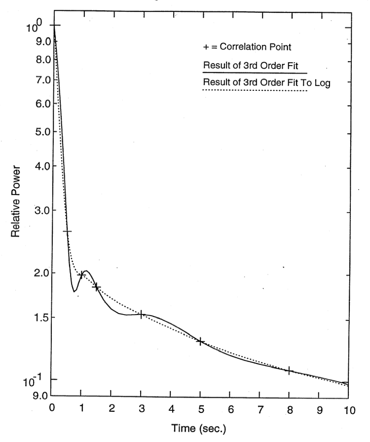
Care should be taken when using third order fits, since they can result in spurious wiggles. Figure 5.16.1 shows the results of a third order fit to the power level in the SHRT-17 test in EBR-II. In this case, the third order fit to the power produces wiggles, whereas the third order fit to the logarithm of the power produces a smooth curve.

Figure 5.16.1 Figure A5.5-1. Fit to SHRT-17 Normalized Total Power, Early Times.