2. SAS4A/SASSYS‑1 User’s Guide¶

2.1. Introduction¶

This chapter contains information that will aid the user in understanding the program architecture of the SAS4A/SASSYS‑1 computer code, and the relationship between its modeling concepts and the program logic and data flow. The code structure is described in terms of modules and subroutines, as are the data management features employed to communicate input and calculated data among modules. The contents and organization of input and output files are described, and results from simplified example problems are included and illustrated.

2.2. Modeling Concepts and Code Structure¶

2.2.1. Code Structure Basis¶

The code structure of SAS4A/SASSYS‑1 is constructed to reflect the physical modeling assumptions employed. In the core models, the basic geometric modeling element is a fuel pin, its cladding, and the associated coolant and structure, with the structure field representing wire wraps, grid plates, and/or hex cans. In the SAS4A/SASSYS‑1 terminology, the term “channel” is used to denote collectively this basic element of fuel, cladding, coolant, and structure. In a single-pin model, a single average channel is used to represent the average of many pins in the reactor, and multiple channels are used to extend the model to all the pins in the reactor. In a multiple-pin model, each channel represents one or more pins in a subassembly, and multiple-pin subassembly models are joined with single-pin subassembly models to cover the whole reactor core. A single SAS4A/SASSYS‑1 channel may therefore represent either one pin, or a large number of pins in many subassemblies. In either case, the elementary unit from a code structure and data management stand-point is an individual channel.

The code structure of SAS4A/SASSYS‑1 is also the result of the programming language employed and the functional requirements of the phenomenological models. The programming language used for SAS4A/SASSYS‑1 is ANSI FORTRAN, and the organization of the code follows the FORTRAN convention of a MAIN program with a number of subroutines and functions. For the purpose of this discussion, the subroutines and functions of SAS4A/SASSYS‑1 are grouped according to purpose into one of the sixteen modules listed in Table 2.2.1. These modules are aligned in a one-to-one fashion with the phenomenological models of SAS4A/SASSYS‑1, each of which is described by a chapter in this report. (The D3IF module is not documented in this report.)

Table 2.2.1 SAS4A/SASSYS‑1 Modules¶
Module	Purpose
ROOT	Logic path control, data management, and material properties services.
TSCL0	Single phase liquid coolant thermal/hydraulics and fuel element heat transfer.
TSPK	Reactor point kinetics and first order perturbation theory reactivity feedbacks.
PRIMAR‑4	Primary and secondary coolant loops and components thermal/hydraulics and heat transfer.
CNTLSYS	Reactor and plant control and protection systems simulation.
BOP	Balance‑of‑plant systems and components thermal/hydraulics and heat transfer.
DEFORM‑4	Oxide fuel/cladding fuel element mechanics.
DEFORM‑5	Cladding mechanics for metallic‑fuel elements.
SSCOMP	Metallic‑fuel pre‑transient characterization and material properties.
FPIN2	Metallic fuel/cladding fuel element mechanics.
TSBOIL	Two‑phase (boiling) coolant thermal/hydraulics and fuel element heat transfer.
CLAP	Molten cladding relocation and heat transfer.
PLUTO2	Post‑cladding‑failure oxide fuel/liquid coolant interactions with fuel/coolant thermal/hydraulics.
PINACLE	Molten metallic fuel relocation and heat transfer prior to cladding failure.
LEVITATE	Post‑cladding‑failure oxide and metallic fuel relocation with fuel/cladding heat transfer.
D3IF	Interface to DIF3D-K for TSPK input data generation or DIF3D‑K space/time neutronics.

The SAS4A/SASSYS‑1 MAIN program calls three subroutines in a module that perform 1) data management initialization, 2) code execution, and 3) data management termination. A flowchart for the MAIN program is shown in Figure 2.2.1. Figure 2.2.2 is a flow diagram for INPDRV, the input driver routine. Figure 2.2.3 and Figure 2.2.4 present flow diagrams for SSTHRM and TSTHRM, the steady-state and transient driver subroutines. The contents of the channel loop in TSTHRM are shown in Figure 2.2.5.

2.2.2. Standard Input Data Reading¶

INPDRV calls subroutine READIN, which reads card images from the ASCII input file (see Section 2.5). A complete description of the contents of the input file is contained in Section 2.8.2. If called for, READIN will call subroutine RESTAR to read a binary restart file (RESTART.bin). Subroutine READIN prints input data card images as they are read. Once all input has been read, subroutine DATOUT prints a copy of the final input deck as card images. If control system input has been provided, subroutine CTLIN3 will perform checking of the input data. Subroutine PMCHEK performs a similar function for input material property data. If specified, subroutine INPEDT will print a formatted version of the input data blocks. Subroutine SSIN01 initializes a number of constants used in the calculations and subroutine PRECAL prepares correlations of metallic fuel material properties (density, specific heat, and thermal conductivity) based on the Integral Fast Reactor Handbook [2‑1, 2‑2], if specified.

Figure 2.2.1 MAIN Program Flow Diagram¶

Figure 2.2.2 INPDRV Subroutine Flow Diagram¶

Figure 2.2.3 SSTHRM Subroutine Flow Diagram¶

Figure 2.2.4 TSTHRM Subroutine Flow Diagram¶

Figure 2.2.5 Flow Diagram for the Channel Loop in TSTHRM¶

A developmental interface to the DIF3D neutron diffusion theory code [2‑3] is provided for by a call to subroutine DATEDT. When fully operational, DATEDT will manage the calculation of the reactor power distribution, reactivity feedback, and point kinetics data for the TSPK module. (Future plans call for implementation of the DIF3D-K space-time neutronics code [2‑4] in SAS4A/SASSYS‑1). Finally, INPDRV calls CRVSUP to supervise the fitting of various input data tables to correlations.

2.2.3. Steady-State Calculation¶

Figure 2.2.3 presents a flow diagram for the steady-state (pre-transient) driver subroutine, SSTHRM. SSTHRM begins by making calls to SSPINT, which initializes data for the multiple-plenum option in PRIMAR‑4, to PNORM, which normalizes the reactor power distribution to the specified condition, and to SSPK, which initializes data for the point kinetics solution module, TSPK. Within a loop over all channels, SSTHRM performs optional initializations for applications of EBR-II thermal/hydraulic uncertainty factors and the multiple-plenum option. Next, an optional path to a single-channel, stand-alone execution of the FPIN2 computer code [2‑5] is provided. Subroutine SSINCH performs channel-dependent data initialization, and subroutine SSFUEL manages the pre-transient thermal, hydraulic, and mechanics calculation for oxide (DEFORM‑4) and metallic (SSCOMP) fuels. (The SSCOMP capability is currently limited to un-irradiated fuel material properties; irradiation effects such as swelling, porosity migration, fission gas generation and release, and fuel/cladding interactions are being added). Should the SSFUEL option not be elected, SSTHRM calls a) subroutine SHAPE to set the axial channel power distribution, b) subroutine SSCOOL to calculate the coolant, structure, and reflector temperatures, c) subroutine SSHTR to calculate the fuel and cladding temperatures, d) subroutine SSPRNT to print the steady-state temperature, geometry, and neutronics results, and e) subroutine NODEPR for an optional diagnostic print of the fuel/cladding temperature calculation. Once all temperatures have been determined, an option is available to apply hot channel factors. If the FPIN2 model is specified for the current channel, subroutine FPINIT provides the interface to the SAS4A/SASSYS‑1 temperature calculation. Subroutine SSPLOT provides an entry for the writing of channel-dependent, steady-state results for subsequent plotting. The final action in the channel loop is optional initialization of data for the multiple-plenum model. Following the channel loop, a summary of the reactor power and flow data for all channels is printed, and the optional subassembly-to-subassembly input data is checked for consistency. If the multiple-pin subassembly model has been invoked, subroutine SSNULL performs a constant power and flow transient calculation to bring the participating channels to an equilibrium temperature condition. If the multiple-plena PRIMAR‑4 option is used, steady-state plena conditions are then set by a call to subroutine SSTOUT. PRIMAR‑4 default values are set in a call to SSPRIM, and the optional primary loop, secondary loop, and balance-of-plant steady-state conditions are set by a call to subroutine SSPRM4. Finally, SSTHRM calls subroutine RESTAR to write a restart file RESTART.dat defining the steady-state condition.

2.2.4. Transient Calculation¶

The flow diagram for subroutine TSTHRM, the transient calculation driver routine, is given in Figure 2.2.4. If the problem is beginning from a restart file, subroutine REINIT is called to perform necessary restart initialization. Next, subroutine INGRFN is called to initialize transient driving conditions from the shared memory segment for the simulator option.

The transient problem time domain is divided into time steps as depicted in Figure 2.2.6. Reactivity feedbacks and solutions to the point kinetics equations are obtained on the main time steps. The primary loop, secondary loop, and balance-of-plant thermal/hydraulics solutions are obtained on the primary loop time step, which is a sub-step of the main time step. Recalculations of the core channel temperatures are carried out on the heat transfer time steps, and solutions of the channel hydraulics equations are obtained on the coolant time steps. The heat transfer time step is a sub-step of the main time step, and the coolant time step is a sub-step of the primary loop time step. A coolant time step may not span the end of a heat transfer time step. Heat transfer and coolant time steps may vary from channel to channel for single-pin modeling, or from subassembly to subassembly for multiple-pin or sub-channel modeling. The time step accounting algorithm maintains consistency among the time step levels while adjusting the various step lengths to preserve power, reactivity, and temperature change limits as set by default or in the input to preserve accuracy.

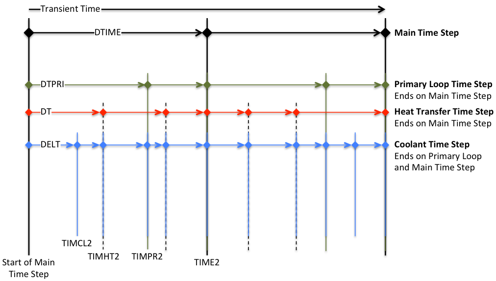
Figure 2.2.6 SAS4A/SASSYS‑1 Time Step Hierarchy¶

Before the first transient main time step, subroutine TSINIT is called to perform initialization. Each main time step begins with a call to subroutine DTMFND to set the time step length, and subroutine FEEDBK is called to initialize the reactivity feedback calculation. For the power vs. time option, subroutine POWING is called to set the reactor power variation over the time step; for the reactivity vs. time option, subroutine POINEX extrapolates the reactivity and subroutine TSPK calculates the reactor power. If the subassembly-to-subassembly heat transfer option has been specified, subroutine CHCHFL is called to calculate the channel-to-channel heat fluxes. The primary loop time step, a substep of the main time step, begins with a call to subroutine DTPFND, which sets the primary loop time step length. Subroutine PRIMAR supervises the thermal/hydraulic calculations for the primary and secondary loops and the balance-of-plant, setting temperature and flow boundary conditions for the core. Subroutine LBPLOT provides optional writing of selected balance-of-plant plotting data on the last primary loop time step in a main time step, and subroutine FEEDBK then retrieves PRIMAR‑4-calculated data for calculation of reactivity feedbacks. At this point, a loop over channels is begun. Optional multiple-plena conditions are set, as is the channel decay heat or power curve. At this point, if the current channel is one of the pins in the multiple-pin subassembly model, but not the first channel, then a skip is made around the subsequent channel thermal/hydraulics driver subroutines (i.e. TSCL0, TSBOIL, LEVDRV, and PLUDRV), since this channel’s thermal hydraulics solution has already been obtained within the multiple-pin model. (At present, the multiple-pin model is limited to single-phase coolant flow, but may be extended to coolant boiling and pin disruption modeling in the future). On the other hand, if this is a single-pin channel or the lead multiple-pin channel, subroutine DTCFND is called to set the coolant time step length (a subset of the primary loop time step and variable from one channel to another in the single-pin model and from one subassembly to another in the multiple-pin model). The channel coolant hydraulics solution is obtained on the coolant time step. TSTHRM then calls one of the channel thermal/hydraulics driver subroutines (TSCL0, TSBOIL, LEVDRV, or PLUDRV), depending on the thermal/hydraulics conditions in the channel. One of these driver subroutines then advances the channel calculation to the end of the current coolant time step, checking the current time along the way to determine whether a recalculation of the pin temperatures is necessary.

At this point in subroutine TSTHRM, a check is made to determine if the current coolant time step has ended on a heat transfer time step. If not, the calculation proceeds to the next coolant time step. If the end of the heat transfer has been reached, newly-determined channel temperatures are available, and this triggers tests on the need for fuel element mechanics (DEFORM‑4, DEFORM‑5, FPIN2) or in-pin fuel relocation (PINACLE) calculations. But first, a test is made to determine whether the input has specified the approach of a fission-gas-plenum cladding failure time, and subsequent gas release into the coolant channel. Next, a check is made to determine whether this channel has experienced cladding failure; if so, subsequent tests for fuel pin mechanics or in-pin fuel relocation are skipped. If cladding failure has not occurred, the PINACLE module is invoked if conditions are met for in-pin fuel relocation, and subroutine FAILUR is called to check for cladding failure. If one of the fuel pin mechanics options has been specified, it is executed at this point. This brings the calculation to the bottom of the primary loop and main time step branches.

At the end of a primary loop time step, a check is made to determine whether the end of the main time step has been reached. If not, another primary loop time step will be made to advance the calculation. However, if the end of the main time step has been reached, a series of tests are made to check for the writing of plotting file data (subroutines PNPICO, LEPICO, and TSPLOT), to sum a channel’s contribution to the net reactivity (subroutine FEEDBK), and to print channel conditions (subroutines TSPRNT and OUTPT5). A test is made to determine whether all channels have been advanced to the end of the primary loop time step; if not, the next channel is calculated, but if so, a test is made on the current time to check for the end of the main time step. If the end of the main time step has not been reached, subsequent primary loop time steps are made until the end of the main time step is found. Then, subroutine FEEDBK is called to total the net reactivity, and for the reactivity vs. time option, subroutines TSPK and RHOEND are called to solve the point kinetics equations over the main time step. If specified, the reactor power and reactivity data are added to the plotting file (entry TSPLT2), and subroutine PKPAGE is called to print the power and reactivity summary page on a time step interval set by input. Subroutine PSHORT produces a short-form power and reactivity print on each time step, followed by tests for problem termination on the basis of computing time limit, maximum number of time steps, maximum problem time, or minimum fuel motion reactivity. If a termination condition is found, a test is made to produce the major channel prints (subroutine TSPRNT) in the event they were not made on the current time step. If a termination condition is not found, the calculation continues following checks for a) the writing of restart file from subroutine RESTAR, b) the optional transfer of data to and from the shared memory segment in conjunction with the simulator option, and c) the optional print of a computing time summary. At termination, the restart file is written automatically and the final computing time summary is printed, followed by the return to program MAIN, where a summary of all subroutines entered in the calculation is printed and execution halts.

2.3. Data Management¶

In order to minimize memory requirements and enhance computational performance, the SAS4A/SASSYS‑1 data management scheme maintains a framework for optional data storage. Accordingly, users have the ability to control data allocation for specific modules via the storage allocation record. These storage flags affect the creation of module-specific data structures that are utilized for management of dynamically allocated memory and common block data.

Flag IADEFC on the storage allocation record affects channel-specific data allocation for DEFORM-4, DEFORM-5, and FPIN2 data, meaning allocation of these data structures is necessary if any of these modules are to be utilized. Flag IAPLUC controls allocation of memory for data related to PINACLE, LEVITATE, or PLUTO2; similar to IADEFC, allocation using IAPLUC is necessary if any the related modules are utilized during a simulation. It should be noted that problems that initiate either PINACLE, LEVITATE, or PLUTO2 must have either DEFORM‑4 or DEFORM‑5 also running, but the DEFORM modules may operate without PINACLE, LEVITATE, or PLUTO2.

Two additional storage areas are allocated for the control system module (CNTLSYS) and the balance-of-plant module (BOP). These areas need not be allocated if the corresponding module is not to be executed. Allocation of the CNTLSYS storage is controlled with variable IACNTL on the storage allocation record, and the BOP module storage area allocation option is controlled with variable IALBOP in the same record.

If the optional SAS4A/SASSYS‑1 interface to the DIF3D code is used, the DIF3D modules allocates two storage areas under the control of the BPOINTR package. These storage areas are used only on the DIF3D side of the interface.

2.4. Supported Platforms¶

Currently, SAS4A/SASSYS‑1 is supported on 64-bit macOS, Linux, and Windows platforms with the x86_64 architecture.

2.5. Input and Output Files¶

2.5.1. SAS Input File¶

In the past, SAS4A/SASSYS‑1 input was limited to 80-column, fixed-formatted card images. This is still the basic format used by most SAS input files. However, Version 5.3 introduces the option to use free-formatted input of any length for integer and floating-point input blocks. A full description of the contents of the input file is contained in Section 2.8.2.

In all SAS input files, the first three (non-comment) records of the input file are required. The first two records each contain 72 columns of problem title data that will appear at the top of each page of the output file. Columns 73‑80 of the first card image must contain, left adjusted, the major and minor version number of the SAS code being executed. The third record is the storage allocation card, which provides SAS information needed to allocate the various data containers used for input processing. If the DIF3D interface option is invoked, an additional storage allocation card (fourth record) is required.

If the current execution is to be restarted from a prior execution, the input file must contain a RESTART directive to invoke the reading of a restart file from RESTART.bin (see Section 2.5.3). The reading of the restart file takes place at the point the restart record is encountered on the input file. Input blocks loaded before the restart record will be over-written by the restart file data, and input blocks following the restart record will modify or replace data read from the restart file.

The input data blocks for SAS are described in Section 2.8.2. Each input data block begins with a block identifier record and ends with a block delimiter record. The block identifier record contains the block name and number, and two integers denoting the relevant current channel and the type of background data fill to be supplied before data reading begins. (The background may be “zeros” or the same block entered previously for this or another channel.) The block delimiter record accepts either a negative integer one (“-1” right adjusted) entered in the first I6 field of the record, or a left adjusted “END” statement.

Within the body of a SAS input file, INCLUDE directives may be used to read additional input data from external files. Any number of nested INCLUDE directives may be used, but circular references are not allowed. Support for INCLUDE directives was added in Version 5.3.

Reading of input is terminated by an ENDJOB directive. Any records following the ENDJOB record are ignored.

2.5.2. SAS Output File¶

SAS4A/SASSYS‑1 prints output as 133-column, formatted, printed line images. Listings of example output files can be found in the example problems output listings provided with the code distribution.

The output file is occasionally divided by logical page breaks. (A fixed page size of 60 lines is no longer maintained.) Each logical page break is headed with the two title records that begin the input deck. The title lines also contain code version identification, the page number, job and user identification, the execution date, and the clock time. Pages containing channel-dependent information will have the channel number printed in the upper left-hand corner.

The output file begins with a print of information from the header, including primary and secondary titles and memory allocation flags. During input processing, each record from the input file is recorded to the file SAS.log. An optional compiled version of the input may be written to INPUT.dat (see IPDECK). An optional, formatted and annotated print of the input data is available, followed by a tabular print of coolant material properties. This is followed by printer plots of curves formed by the tabular fitting procedure.

The steady-state results are printed next, beginning with prints of channel-dependent data. The prints vary depending on the computational modules invoked, but usually contains node-wise masses, porosities, and temperatures, as well as radial and axial pin geometry. Also printed are nodal powers and reactivity feedback coefficients. Following the channel-dependent prints, steady-state results from the primary loop (PRIMAR‑4), control system, and balance-of-plant may appear, if those modules are employed.

A short print of time, power, and reactivity is produced on each main transient time step. The exact form of this print varies depending on whether the default reactivity feedback routines are employed or the EBR-II feedback routines are used. On specified main time steps, long prints of the current channel conditions (geometry, pressure, temperature, etc.) are produced. In addition, each module may produce intermittent transient prints of calculated results. These prints are controlled by input data. Extensive diagnostic prints may also be triggered through input for most of the computational modules.

2.5.3. Auxiliary Input and Output Files¶

The input and output files used in SAS4A/SASSYS‑1 are listed in Table 2.5.1.

Table 2.5.1 SAS4A/SASSYS‑1 Assigned External Files¶
File	Type	Assigned Use	Subroutine
stdin	Formatted	Input Data Records	READIN
stdout	Formatted	Printed Output	READIN
			DATOUT
			SSPRNT
			TSPRNT
			PSHORT
			PKPAGE
INPUT.dat	Formatted	Edited Input Data Records	DATOUT
8	Formatted	Scratch BOP Input Data	READIN
			RENUM
SAS.log	Formatted	Printed Output
CHANNEL.dat	Binary	Main Time Step Plotting	TSPLOT
12	Binary	PLUTO2/LEVITATE Data for Plotting	PLOUT
13	Binary	PLUTO2/LEVITATE Data for Plotting	PLOUT
14	Binary	PLUTO2/LEVITATE Data for Plotting	PLOUT
PRIMAR4.dat	Binary	PRIMAR‑4 Data for Plotting	SSPRPL
			TSPRPL
CONTROL.dat	Binary	Control System Signal Data	CNTL_Data
16	Formatted	PINACLE/LEVITATE Data for Plotting	SSPLOT
			PNPICO
			LEPICO
RESTART.dat	Binary	Output Restart File	RESTAR
RESTART.bin	Binary	Input Restart File	RESTAR
20	Binary	TSBOIL Data for Plotting	TSCMP0
			TSCMP1
21	Binary	DEFORM‑5 Plotting	DFORM5
22	Binary	EBR2 Reactivity Plotting	EBR2
23	Binary	FPIN2 Data for Plotting	FPNOUT
24	Binary	EBR-II Mark-V Safety Case Scratch Plotting Data File	TSPLOT
26	Binary	BOP Data for Plotting	LBPLOT
27	Binary	Steam Generator Data for Plotting	INIT, TSBOP
28	Binary	BOP Data for Plotting	INITS, TSBOP
29	Binary	BOP Data for Plotting	PLTBOP
MaxTemps.txt	Formatted	Summary of Maximum Temperatures in the Core	PRTMXT

2.6. Example Problems¶

2.6.1. Protected Transient Overpower Example Problem¶

The protected transient overpower example problem, which is distributed with SAS4A/SASSYS‑1 releases as “exam1”, is an analysis of a protected reactivity insertion event in the EBR‑II reactor. The basic SAS4A/SASSYS‑1 input deck for this example problem was taken from Ref. 2‑6. This input deck is the standard EBR‑II SAS4A/SASSYS‑1 model for the primary and secondary coolant loops. The core model in this deck is for a generic Mark‑III reactor, and does not correspond to an actual or planned loading. The standard EBR‑II plant protection system model documented in Ref. 2‑7 was added to the input deck to provide scram functions, and an external, programmed reactivity insertion of 0.01 $/second to a maximum of 0.15 $ was assumed to drive the transient beginning from the steady‑state conditions.

The input reactivity insertion raises the reactor power to 115% of nominal. At this power level, the plant protection system begins a reactor scram sequence by inserting a total of ‑3.7 $ of reactivity over 0.45 seconds, sharply reducing the power. Six seconds following the scram signal, a manual trip of both primary coolant pumps is assumed, followed six seconds later by a manual trip of the secondary pump. (The primary pump trip is not standard EBR-II operating practice, but is assumed here for the purpose of demonstrating SAS4A/SASSYS‑1). The auxiliary pump continues to operate throughout the sequence.

The reactor power history and the flow history in channel 3, a high‑power driver subassembly, are plotted in Figure 2.6.1. The power reduction begins at ten seconds, and the core flow reduction begins at approximately sixteen seconds. Over the next two minutes, the power drops to the decay heat level, and the flow seeks an equilibrium at the level provided by the auxiliary pump and natural circulation.

The peak fuel, cladding, and coolant temperature histories in channel 3 are plotted in Figure 2.6.2, along with the coolant saturation temperature. The fuel, cladding, and coolant temperatures rise with the power until the reactor scram. Temperatures then drop with the falling power, until the primary pumps are tripped and the flow reduction causes the temperatures to rise. The coolant saturation temperature falls as the coolant pressure drops during the coast-down of the two primary pumps. As the coolant temperature rises, the increased buoyancy causes the reactor coolant flow to increase slightly, until at about 45 seconds into the transient, a local temperature maximum occurs, at a level near the initial peak cladding temperature. From this time forward, temperatures slowly fall as the coolant flow adjusts to the combination of forced and natural circulation at decreasing decay heat power.

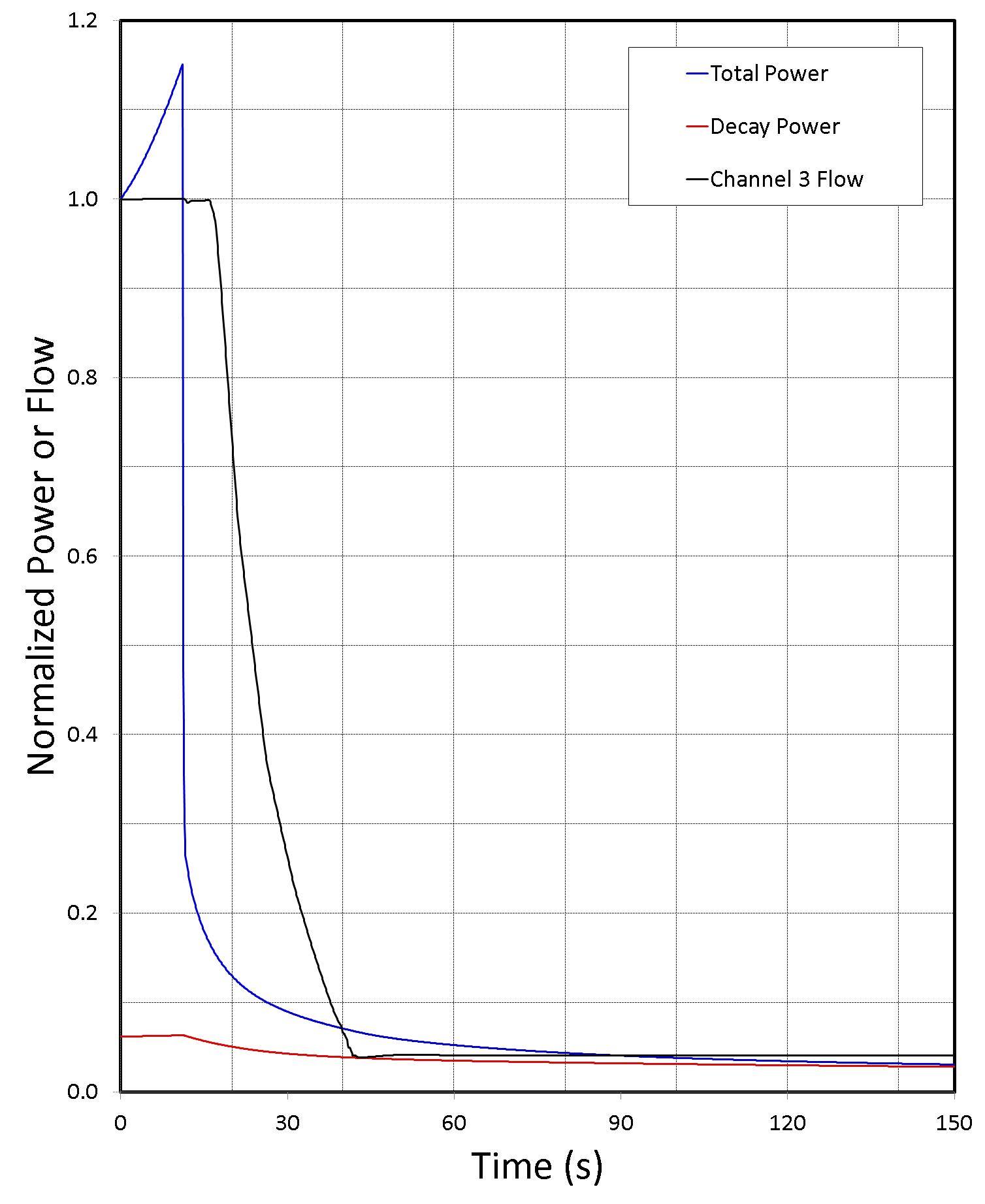
Figure 2.6.1 SAS4A/SASSYS‑1 Reactor Power and Flow Histories¶

Figure 2.6.2 SAS4A/SASSYS‑1 Temperature Histories in the High Temperature Driver Subassembly¶

2.6.2. Unprotected Transient Overpower Example Problem¶

The unprotected transient overpower example problem, which is distributed with SAS4A/SASSYS‑1 releases as “exam2”, is an analysis of an unprotected (without scram) transient overpower (TOP) accident in a metal-fueled 3500 MWt pool-type reactor. This reactor has been analyzed previously for accident initiators that included unprotected loss-of-flow (LOF) and loss-of-heat-sink (LOHS) sequences as well as the transient overpower sequence [2-8]. However, the TOP sequence analyzed previously corresponded to removal of one control rod. For this analysis, the ramp reactivity addition rate was set to 0.10 $/s, and no limit was placed on the total reactivity added. This ramp rate results in an initial reactor power rise that approximately corresponds to the 8-second period employed in the TREAT M-Series tests [2-9], and the unlimited insertion assures that fuel melting and cladding failure will occur. Therefore, the whole-core sequence demonstrates 1) molten metal fuel behavior at conditions similar to those of the TREAT M-Series tests, 2) the ability of the SAS4A/SASSYS‑1 metal fuel relocation modules, PINACLE and LEVITATE, to reproduce metal fuel performance observed in TREAT, and 3) the reactor safety implications of TREAT fuel relocation observations.

The TOP sequence assumed here is an unlimited 0.1 $/s reactivity ramp addition with failure of the plant protection and safety systems. It is also assumed that since no scram takes place, the reactor coolant pumps continue to operate. The reactor power history calculated by SAS4A/SASSYS‑1 for this sequence is shown in Figure 2.6.3, and the corresponding net and component feedback reactivities are shown in Figure 2.6.4.

As shown in Figure 2.6.3, the reactor power rises initially in response to the ramp reactivity insertion, which is labeled as “Program” in Figure 2.6.4. The initial power ascension approximates the TREAT M-Series 8-second period. At about 7 seconds into the transient, conditions for in-pin fuel relocation are satisfied, and the PINACLE model begins execution to describe the expulsion of fuel within the cladding from the core into the fission gas plenum region, first for a few subassemblies and for more of the core as time goes on. This fuel relocation provides a negative reactivity effect that reduces the power temporarily, countering the input ramp reactivity.

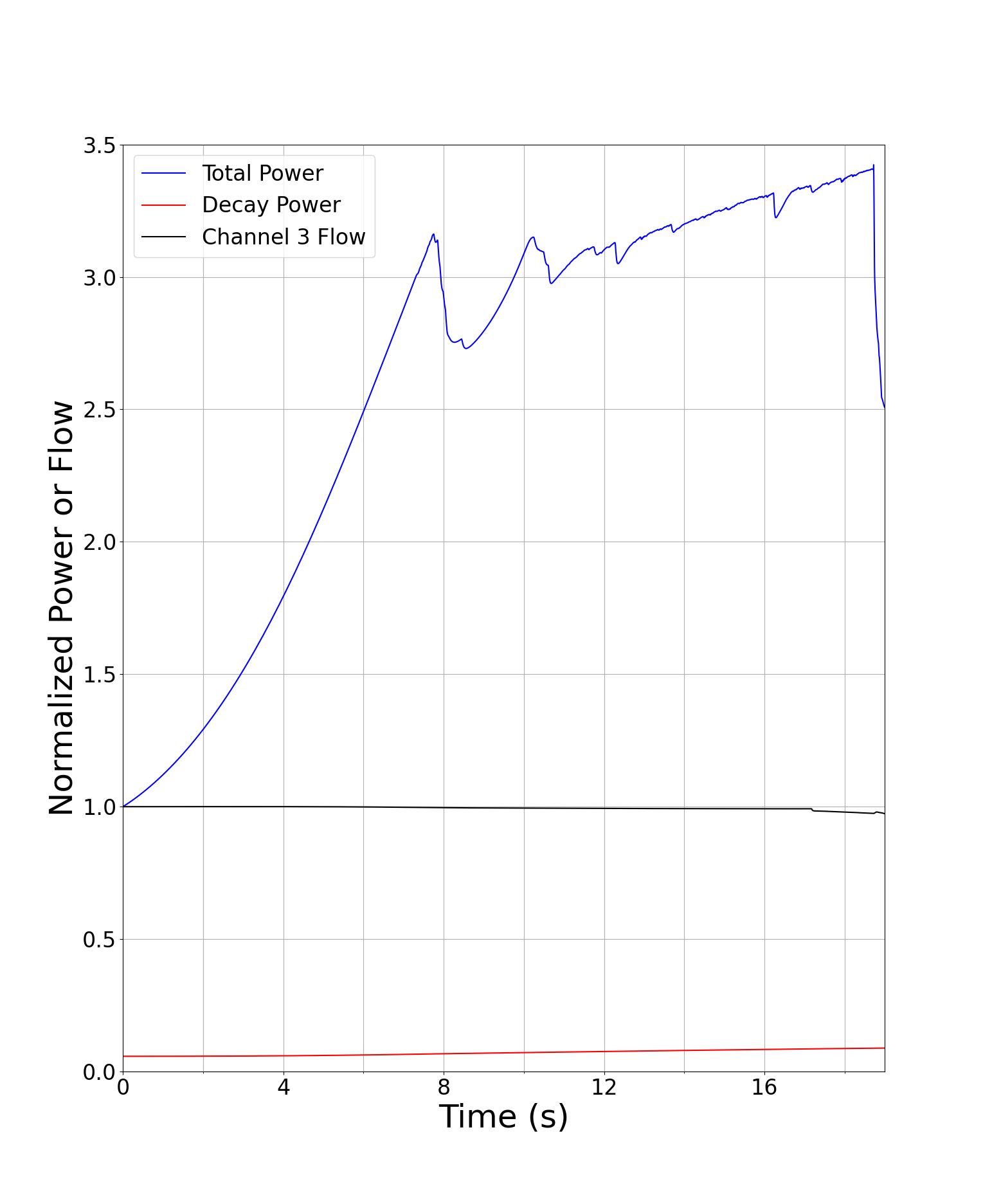
Figure 2.6.3 SAS4A/SASSYS‑1 Example Problem Reactor Power History¶

Figure 2.6.4 SAS4A/SASSYS‑1 Example Problem Reactivity History¶

2.7. References¶

2-1. G. L. Hofman, et al., Unpublished information, Argonne National Laboratory, 1985.

2-2. IFR Properties Evaluation Working Group, “Handbook of Properties of Metallic Fuels,” Argonne National Laboratory, Idaho Falls, Idaho, June, 1988.

2-3. K. L. Derstine, Unpublished information, Argonne National Laboratory, 1984.

2-4. T. A. Taiwo and H. S. Khalil, “The DIF3D Nodal Kinetics Capability in Hex‑Z Geometry ‑ Formulation and Preliminary Tests,” Proceedings of the International Topical Meeting Advances in Mathematics, Computations, and Reactor Physics, American Nuclear Society, Pittsburgh, Pennsylvania, April 28 ‑ May 2, 1991.

2-5. T. H. Hughes and J. M. Kramer, “The FPIN2 Code ‑ An Application of the Finite Element Method to the Analysis of the Transient Response of Oxide and Metal Fuel Elements,” Conference on the Science and Technology of Fast Reactor Safety, British Nuclear Energy Society, Guernsey, May 12 ‑ 16, 1986.

2-6. J. P. Herzog, Unpublished information, Argonne National Laboratory, 1993.

2-7. J. Y. Ku and T. C. Hung, Unpublished information, Argonne National Laboratory, 1992

2-8. R. A. Wigeland, R. B. Turski, and R. K. Lo, Unpublished information, Argonne National Laboratory, 1990.

2-9. T. H. Bauer, “Behavior of Modern Metallic Fuel in TREAT Transient Overpower Tests,” Nucl. Tech., vol. 92, p. 325, December, 1990.

2-10. “Function Parser for C++ v4.5.1,” http://warp.povusers.org/FunctionParser

2-11. “Function Parser for C++ v4.5.1: Documentation,” http://warp.povusers.org/FunctionParser/fparser.html#functionsyntax