11.2. Fuel Element Mechanics

The mechanical model of FPIN2 uses an implicit finite element method based on a force-displacement formulation. The elements are defined by dividing the fuel and cladding into a number of axial segments and radial rings. Axial symmetry of the loads and generalized plane strain are assumed; therefore, the elements are allowed to interact only at the radial boundaries (nodes). The displacements within the elements are approximated by linear functions.

The mechanical analysis of FPIN2 basically provides the fuel and cladding stresses, $\sigma$, and nodal displacements, $\delta$, for each element during overpower and undercooling events. The fuel and cladding behavior model includes thermal expansions, elastic/plastic/creep deformations, cracking, and melting. A continuous cracking model is used in which an element is assumed to crack in the radial direction when the tensile stress exceeds the fracture stress. Pre-existing cracks are also handled by specifying initial crack strains.

The finite element equilibrium equations are derived from equations of virtual work that leads to a force balance between the external and internal forces

(11.2-1) $$\underline{f}^{\text{int}}\left( \sigma \right) = \underline{f}^{\text{ext}}$$

The external source vector in this equation, $\underline{f}^{\text{ext}}$, describes the external loads at the cavity boundary and the cladding outer surfaces, and the internal force vector, $\underline{f}^{\text{int}} \left( \sigma \right)$, depends on the unknown stress field that must be found to satisfy Eq. (11.2-1) and the constitutive laws for the materials. When this generally non-linear set is linearized and the equations for both the fuel and cladding elements are assembled together for the unknown nodal displacements at each axial segment, the resulting linear equation set can be written symbolically as

(11.2-2) $$\left\lbrack K \right\rbrack \underline{\delta} = \underline{f}$$

where $\left\lbrack K \right\rbrack$ is the stiffness matrix. An elastic-plastic approximation is used in FPIN2 to derive the elements of the stiffness matrix involving the total derivatives of the constitutive equations. The force vector in Eq. (11.2-2) includes the external loads, thermal and other initial strains, and pseudo-forces involving approximations to the plastic and/or creep strains.

The equilibrium equations, Eq. (11.2-1), and the linear equations, Eq. (11.2-2), are solved iteratively for each axial segment by making use of residuals. In this scheme, first the stiffness matrix, $\left\lbrack K \right\rbrack$, and an initial guess for the force vector, $\underline{f}_{0}$, are assembled using available information from the previous time step. Then, the linear equations Eq. (11.2-2) are solved for the new nodal displacements, and from them the increments of total strain are obtained. Assuming that the total material strain is a superposition of elastic, plastic, thermal, and swelling strains, the elastic component of the increments of total strain is separated (see Section 11.2.2) and used to calculate the stress field throughout the fuel element that satisfies the material constitutive equations. These stresses, then, are used to obtain the residuals form the equilibrium equations, Eq. (11.2-1), as follows

(11.2-3) $$\underline{r}_{\text{n}} = \underline{f}^{\text{ext}} - \underline{f}^{\text{int}}\left( \sigma_{\text{n}} \right)$$

where $n$ is the iteration index. Using these residuals, the initial estimate for the force vector in linear equations Eq. (11.2-2) is modified according to

(11.2-4) $$\underline{f}_{\text{n} + 1} = \underline{f}_{\text{n}} + \underline{r}_{\text{n}}$$

The procedure is repeated until convergence is established. This basic scheme is generalized in FPIN2 to include analysis of additional material performance in fuel and cladding such as cracking and melting.

The details of this procedure described above are given in the following sections. The basic stress, strain, and nodal displacement relationships are discussed in Section 11.2.1, and the algorithm for separating elastic strain from the total strain is presented in Section 11.2.2. FPIN2 uses a continuous cracking model that permits cracks in the radial plane. The principles of this model are described in Section 11.2.3. The finite element formulation and the details of the implicit solution scheme outlined above are presented in Section 11.2.4. The formulations given in the aforementioned sections are based on updated geometry and can handle large strains. This is accomplished by performing the mechanics calculation on an incremental basis and updating the fuel element geometry at the end of each time step as described in Section 11.2.5.

11.2.1. Basic Stress-Strain-Displacement Equations

In this section, a number of definitions and basic equations relating stresses, strains, and modal displacements are collected and presented in a uniform notation. These equations constitute the foundation of FPIN2’s mechanics model and serve as the basis for derivations in later sections. Formulas are derived for large-strain finite element analysis of deformation in a cylindrical fuel element under accident conditions. At the beginning of the analysis, the fuel element is assumed to be stress-free with steady-state thermal conditions. Thermoeleastic-plastic behavior is assumed for both the fuel and cladding. Swelling (including hot-pressing) and cracking are also allowed in both materials.

Fuel elements are assumed to consist of a number of axial segments. The finite elements are defined in each axial segment separately and allowed to interact only at the radial boundaries (nodes). The displacements within the elements are approximated by linear functions of the nodal displacements. Axial symmetry of temperatures and external loads is assumed; therefore, the finite elements can be viewed as a series of concentric annular rings. The generalized plane strain assumption is used describe the interaction between the axial segments.

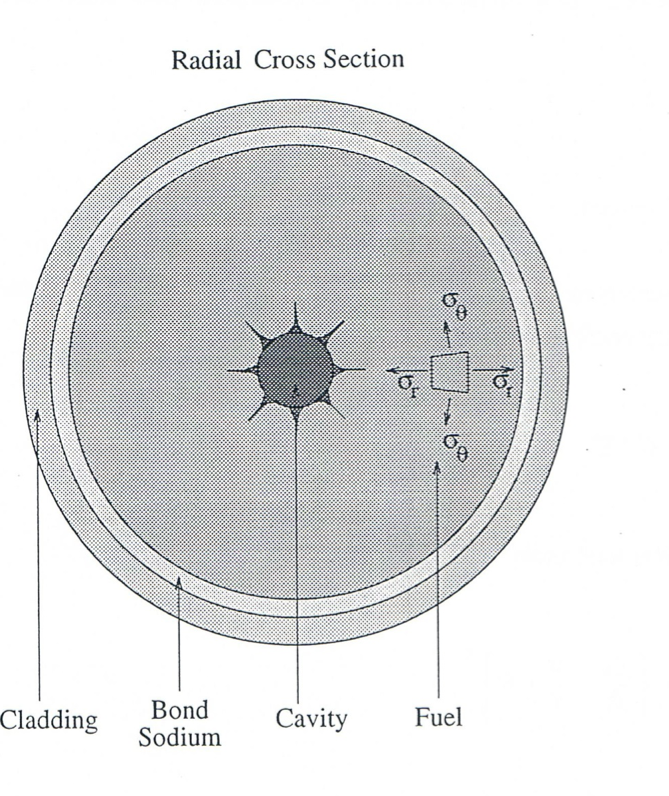
Figure 11.2.1 FPIN2 Geometry

Each axial segment is allowed to have regions containing central cavity gas and/or molten fuel, regions of solid material that are uncracked, and regions that contain radial cracks (Figure 11.2.1). If an element does not contain any cracks, the axisymmetry assumption dictates that the deformation depends only on $r$. Although the existence of radial cracks, in general, destroys this symmetry, it is assumed that the number of cracks in an element is large enough to make the deformation essentially axisymmetric.

11.2.1.1. Strain-Displacement Relationships

In cylindrical coordinates, the strain-displacement relations are given by

(11.2-5) $$\underline{\varepsilon}^{t} = \left\{ \varepsilon_{\text{r}}^{t}, \varepsilon_{\theta}^{t}, \varepsilon_{\text{z}}^{t} \right\}^{T} = \left\{ \frac{\partial \text{u}}{\partial \text{r}} , \frac{u}{r} + \frac{1}{r} \frac{\partial \text{v}}{\partial\theta} , \frac{\partial \text{w}}{\partial \text{z}} \right\}^{T}$$

where $u, v$, and $w$ are displacements in $r, \theta$ and $z$ coordinate directions, respectively. If the material is continuous, the deformation depends only on $r$ due to axisymmetry of temperatures and loads. If the material contains radial cracks, the tangential displacement, $v$, can be expressed as a linear function of $\theta$ in a first order approximation assuming that sufficiently numerous radial cracks exist in the element. In the axial direction, the generalized plane strain condition requires that

(11.2-6) $$w = \psi z$$

where $\psi$ is a constant.

For convenience, we may rewrite the strain-displacement relation as follows to differentiate the crack strain from continuous material strain

(11.2-7) $$\underline{\varepsilon}^{t} = \underline{\varepsilon}^{a} + \underline{\varepsilon}^{c}$$

where “apparent total strain” and “crack strain” vectors are given respectively by

(11.2-8) $$\underline{\varepsilon}^{a} = \left\{ \frac{\text{du}}{\text{dr}} , \frac{u}{r} , \psi \right\}^{T}$$

(11.2-9) $$\underline{\varepsilon}^{c} = \left\{ 0, \varepsilon_{\theta}^{c}, 0 \right\}^{T}$$

Here, $\underline{\varepsilon}_{\theta}^{c}$ is the unknown crack strain component related to radial creaks in the material.

11.2.1.2. Components of Total Strain

The total material strain, $\underline{\varepsilon}^{t}$, can be written as the sum of the elastic strain, $\underline{\varepsilon}^{e}$, the plastic strain, $\underline{\varepsilon}^{p}$, the thermal strain, $\underline{\varepsilon}^{\theta}$, and the swelling strain, $\underline{\varepsilon}^{s}$:

(11.2-10) $$\underline{\varepsilon}^{t} = \underline{\varepsilon}^{e} + \underline{\varepsilon}^{p} + \underline{\varepsilon}^{\theta} + \underline{\varepsilon}^{s}$$

11.2.1.2.1. Elastic Strain

In linear elasticity, the components of elastic strain are related to normal stresses through the generalized Hook’s law

(11.2-11) $$\underline{\sigma} = \left\lbrack C \right\rbrack \underline{\varepsilon}^{e}$$

where the matrix $\left\lbrack C \right\rbrack$ is given in terms of Young’s modulus, $E$, and Poisson’s ratio, $\nu$, as follows

(11.2-12) $$\begin{split}\left\lbrack C \right\rbrack = \frac{E\left( 1 - \nu \right)}{\left( 1 + \nu \right) \left( 1 - 2\nu \right)}\ \begin{bmatrix} 1 & \frac{\nu}{\left( 1 - \nu \right)} & \frac{\nu}{\left( 1 - \nu \right)} \\ \frac{\nu}{\left( 1 - \nu \right)} & 1 & \frac{\nu}{\left( 1 - \nu \right)} \\ \frac{\nu}{\left( 1 - \nu \right)} & \frac{\nu}{\left( 1 - \nu \right)} & 1 \end{bmatrix}\end{split}$$

In general, the elastic parameters $E$ and $\nu$ are functions of temperature, $T$.

11.2.1.2.2. Thermal Strain

In the original oxide fuel version of FPIN2, the components of isotropic thermal strain, $\underline{\varepsilon}^{\theta}$, are expressed in terms of mean thermal expansion coefficient, $\alpha_{\text{m}}$, as follows

(11.2-13) $$\varepsilon_{\text{r}}^{\Theta} = \varepsilon_{\theta}^{\Theta} = \varepsilon_{\text{z}}^{\Theta} = \alpha_{\text{m}} \left( T - T_{0} \right)$$

where $T_{0}$ is a reference temperature. In more recent applications for metallic fuels, the thermal expansion is expressed in terms of handbook linear thermal expansion data [11-7], $\Delta L/L_{0}$, as discussed in Section 11.3.3. Using the thermal data provides more detailed information since it automatically includes the total fuel expansion at solid-to-solid phase transitions. Any other stress-independent isotropic swelling strains (such as selling due to solid fission products or small surface tension dominated gas bubbles) are treated in the same manner as thermal strains in the model.

11.2.1.2.3. Swelling strain

Stress dependent swelling strains, $\underline{\varepsilon}^{s}$, due to fission gas in the fuel are also assumed to be isotropic and required to be expressed by an implicit function of the form

(11.2-14) $$g \left( \sigma_{\text{m}}, \varepsilon^{s}, \frac{\text{d}\varepsilon^{s}}{\text{dt}}, T, \nabla T, \rho \right) = 0$$

Here, the mean hydrostatic stress $\sigma_{\text{m}}$ is calculated from

(11.2-15) $$\sigma_{\text{m}} = \frac{\sigma_{\text{r}} + \sigma_{\theta} + \sigma_{\text{z}}}{3}$$

Hot-pressing is also considered in the model as a negative contribution to the total swelling.

11.2.1.2.4. Plastic strain

The plastic deformation of the material is postulated to occur when a generalized von Mises flow condition is satisfied:

(11.2-16) $$f\left( \sigma_{\text{e}}, {\overline{\varepsilon}}^{p}, \frac{d{\overline{\varepsilon}}^{p}}{\text{dt}} , T \right) = 0$$

where the equivalent stress, $\sigma_{\text{e}}$, and equivalent plastic strain, ${\overline{\varepsilon}}^{p}$, are given respectively by the following equations

(11.2-17) $$\sigma_{\text{e}} = \sqrt{\frac{3}{2}\left( S_{\text{r}}^{2} + S_{\theta}^{2} + S_{\text{z}}^{2} \right)}$$

(11.2-18) $${\overline{\varepsilon}}^{p} = \int{d{\overline{\varepsilon}}^{p}} = \int{\sqrt{\frac{2}{3}\left\lbrack \left( d\varepsilon_{r}^{p} \right)^{2} + \left( d\varepsilon_{\theta}^{p} \right)^{2} + \left( d\varepsilon_{z}^{p} \right)^{2} \right\rbrack}}$$

with the deviatoric stresses defined as

(11.2-19) $$S_{\text{i}} = \sigma_{\text{i}} - \sigma_{\text{m}}$$

$\left( i = r, \theta, z \right)$. The normality condition of plasticity states that the increment of the plastic strain is proportional to the gradient in stress space of the flow condition:

(11.2-20) $$\underline{\text{d}\varepsilon}^{p} = \text{d}\lambda \underline{W}$$

where $\text{d}\lambda$ is the proportionality factor. The gradient vector is given by

(11.2-21) $$\underline{W} = \left\{ \frac{\partial\sigma_{\text{e}}}{\partial\sigma_{\text{r}}} ,\frac{\partial\sigma_{\text{e}}}{\partial\sigma_{\theta}} , \frac{\partial\sigma_{\text{e}}}{\partial\sigma_{\text{z}}} \right\}^{T} = \frac{3}{2\sigma_{\text{e}}}\left\{ S_{\text{r}}, S_{\theta}, S_{\text{z}} \right\}^{T}$$

For the particular form of flow conditions chosen in this model, the factor of proportionality, $\text{d} \lambda$, is identical to the increment in equivalent plastic strain, $\text{d}{\overline{\varepsilon}}^{p}$. The plastic strains are assumed to occur with zero volume change:

(11.2-22) $$\varepsilon_{\text{r}}^{p} + \varepsilon_{\theta}^{p} + \varepsilon_{\text{z}}^{p} = 0$$

The constitutive equations for plastic deformation as well as swelling (Eq. (11.2-16) and Eq. (11.2-14)) indicate that, in general, the deformation depends on the changes in stress and temperature. Also, a major part of the deformation in a fuel element at high temperatures is rate dependent. The discussion of the material properties for the swelling and plastic behavior of the metallic fuel pins is given in Section 11.3.

11.2.1.3. Incremental Stress-Strain Relationships

Since the elastic constants of the matrix $\left\lbrack C \right\rbrack$ in Eq. (11.2-11) are functions of temperature, $T$, the incremental elastic stress components are given by

(11.2-23) $$\underline{\text{d}\sigma} = \left\lbrack C \right\rbrack \underline{\text{d}\varepsilon}^{e} + \frac{d\left\lbrack C \right\rbrack}{\text{dT}}{\underline{\varepsilon}}^{e} \text{dT} \ = \left\lbrack C \right\rbrack \left( \underline{ \text{d}\varepsilon^{e} - \frac{ \text{d} \left\lbrack C \right\rbrack^{-1}}{\text{dT}} \underline{\sigma} \text{dT}} \right)$$

Using the equation representing the superposition of strains:

(11.2-24) $$\underline{\text{d}\varepsilon}^{e} = \underline{\text{d}\varepsilon}^{t} - \underline{\text{d}\varepsilon}^{p} - \underline{\text{d}\varepsilon}^{\theta} - \underline{\text{d}\varepsilon}^{s}$$

and replacing $\underline{\text{d}\varepsilon}^{p}$ with equivalent plastic strain increments, the change in stress can be expressed in terms of increment of total strain as follows

(11.2-25) $$\underline{\text{d}\varepsilon} = \left\lbrack C \right\rbrack \left( \underline{\text{d}\varepsilon}^{t} - \underline{W}d{\overline{\varepsilon}}^{p} - \underline{Q}\text{d}T - \underline{\text{d}\varepsilon}^{s} \right)$$

where, for convenience, the thermal modulus $\underline{Q}$ has been introduced:

(11.2-26) $$\underline{Q} = \underline{\alpha} + \frac{\text{d}\left\lbrack C \right\rbrack}{\text{dT}}^{- 1} \underline{\sigma}$$

The mechanical model of FPIN2 makes use of Eq. (11.2-25) to calculate approximate changes in stress given the estimates of plastic and swelling strain increments.

11.2.1.4. Element Types

The actual form of Eq. (11.2-25) depends on the type of fuel element considered. Originally, four different types of elements are considered in the finite element formulation of FPIN2 that allows analysis of cracks in both radial and transverse planes. However, only two types of elements are available in the metal fuel version because cracks in metallic fuels, if they occur, are predominantly radial. The definitions of the two types are as follows:

Type I: The element lies in continuous fuel or cladding. Both the axial and tangential crack strains are zero; therefore, the total stain in the element is equal to the apparent total strain. The resultant of the axial stress is also assumed to be known. [4]

Type II: The element lies in a portion of the fuel where only radial cracks are present and the tangential crack strain is non-zero. The circumferential stress is constant everywhere in the element and equal to the boundary value $\sigma_{\theta} = - p_{\text{g}}$ ($p_{\text{g}}$ is the pressure of the fission gas present in the crack opening.) As in Type I, the resultant axial force is assumed to be known.

Table 11.2.1 Source of Calculated Stress and Strain Results for the Element Types

Element Type	Equilibrium and Strain-Displacement Equations	Crack Strain Definition	Stress Boundary Conditions	Algorithm Described in Section 11.2.2
I	Continuous	$\varepsilon_{\text{r}}^{a} , \varepsilon_{\theta}^{a} , \varepsilon_{\text{z}}^{a}$	$\varepsilon_{\theta}^{c} = 0$	—	$\sigma_{\text{r}} , \sigma_{\theta} , \sigma_{\text{z}}$
II	Radial cracks	$\varepsilon_{\text{r}}^{a} , \varepsilon_{\theta}^{a} , \varepsilon_{\text{z}}^{a}$	$\varepsilon_{\theta}^{c} \neq 0$	$\sigma_{\theta} = - p_{\text{g}}$	$\sigma_{\text{r}} , \sigma_{\text{z}} , \varepsilon_{\theta}^{c}$

In each case, solving the finite element equilibrium equations gives the radial displacement, $u \left( r \right)$, from which apparent strain, $\underline{\varepsilon}^{a}$, can be calculated. The stress and strain components not obtained from the equilibrium equations, strain-displacement relations, or stress boundary conditions are calculated by an algorithm to separate elastic strain from the total strain as described in Section 11.2.2 (see Table 11.2.1).

11.2.1.5. Relationships for Stress Increments: Pseudo-Stress

Since the actual form of Eq. (11.2-25) depends on the type of fuel element considered, it can be expressed in following generalized form

(11.2-27) $$\underline{\text{d}\sigma} = \left\lbrack C \right\rbrack \underline{\text{d}\varepsilon}^{a} - \underline{\text{d}\sigma}^{\text{ps}}$$

where $\underline{\text{d}\sigma}^{\text{ps}}$ is the incremental pseudo-stress. Ad described in Section 11.2.4.2, given the estimates of plastic and swelling strain increments, this pseudo-stress term is treated as a constant within a time step. In other words, Eq. (11.2-27) expresses the changes in stress in terms of a known term $\underline{\text{d}\sigma}^{\text{ps}}$ and an unknown increment $\underline{\text{d}\varepsilon}^{a}$. The calculated stress increments are then corrected to satisfy the equilibrium and constitutive equations to a desired accuracy as described in Section 11.2.4.2.

Existence of radial cracks in the element alters the form of the elastic modulus, $\left\lbrack C \right\rbrack$, and the pseudo-stress vector, $\underline{\text{d}\sigma}^{\text{ps}}$. As shown in Table 11.2.1, for an uncracked element all three components of the total apparent strain are to be found from the equilibrium equations. Therefore, the incremental stress can be written in the form of Eq. (11.2-27) as

(11.2-28) $$\underline{\text{d}\sigma} = \left\lbrack C \right\rbrack \underline{\varepsilon}^{a} - \underline{\text{d}\sigma}_{\text{I}}^{\text{ps}}$$

where $\left\lbrack C_{\text{I}} \right\rbrack$ and the incremental pseudo-stress are simply defined by

(11.2-29) $$\left\lbrack C_{\text{I}} \right\rbrack = \left\lbrack C \right\rbrack$$

and

(11.2-30) $$\underline{\text{d}\sigma}_{\text{I}}^{\text{ps}} = \left\lbrack C \right\rbrack \left( \underline{Q} \text{dT} + \underline{W} \text{d}{\overline{\varepsilon}}^{p} + \underline{\text{d}\varepsilon}^{s} \right)$$

For an element with radial cracks (Type II), Table 11.2.1 indicates that

(11.2-31) $$\underline{\text{d}\varepsilon}^{c} = \left\{ 0 , d\varepsilon_{\theta}^{c} , 0 \right\}^{T}$$

(11.2-32) $$\underline{\text{d}\sigma} = \left\{ \text{d}\sigma_{\text{r}} , - \text{dp}_{\text{g}} , \text{d}\sigma_{\text{z}} \right\}^{T}$$

By substituting these equations into Eq. (11.2-25) and premultiplying by $\left\lbrack C \right\rbrack^{-1}$, $\text{d}\varepsilon_{\theta}^{c}$ can be eliminated and the equations can be solved for $\text{d}\sigma_{\text{r}}$ and $\text{d}\sigma_{\text{z}}$. The result can be written in the form of Eq. (11.2-28) as

(11.2-33) $$\underline{\text{d}\sigma} = \left\lbrack C_{\text{II}} \right\rbrack \underline{\text{d}\varepsilon}^{a} - \underline{\text{d}\sigma}_{\text{II}}^{\text{ps}}$$

where for Type II elements

(11.2-34) $$\begin{split}\left\lbrack C_{\text{II}} \right\rbrack = \frac{E}{1 - \nu^{2}}\begin{bmatrix} 1 & 0 & \nu \\ 0 & 0 & 0 \\ \nu & 0 & 1 \end{bmatrix}\end{split}$$

and

(11.2-35) $$\begin{split}\underline{\text{d}\sigma}_{\text{II}}^{\text{ps}} = \frac{E}{1 - \nu^{2}}\begin{bmatrix} 1 & 0 & \nu \\ 0 & 0 & 0 \\ \nu & 0 & 1 \\ \end{bmatrix}\begin{Bmatrix} W_{\text{r}}\text{d}{\overline{\varepsilon}}^{p} + Q_{\text{r}} \text{dT} + \text{d}\varepsilon^{s} + \frac{\nu \text{dp}_{\text{g}}}{E} \\ \frac{\left( 1 - \nu^{2} \right)\text{d}p_{\text{g}}}{E} \\ W_{\text{z}}\text{d}{\overline{\varepsilon}}^{p} + Q_{\text{z}} \text{dT} + d\varepsilon^{s} + \frac{\nu \text{dp}_{\text{g}}}{E} \end{Bmatrix}\end{split}$$

The singularity of $\left\lbrack C_{\text{II}} \right\rbrack$ reflects the fact that the radial displacements of the inner and outer radii of a cracked element cannot be determined uniquely from its exterior loads. This is due to the reason that a rigid body radial displacement of an element is a possibility. However, when all of the element stiffness matrices for an axial segment are assembled together, the resulting global stiffness matrix is, in general, non-singular and a unique solution for the displacements can be found.

11.2.2. Algorithm for Separating the Components of the Total Strain

In FPIN2, first the finite element equilibrium equations (described in Section 11.2.4.2) are solved to obtain the increments of total apparent strain. After separating the elastic contribution through the use of algorithm described below, we can then calculate the stresses from Eq. (11.2-11). The algorithm, which is based on a method developed by Schreyer [11-8], also yields the other components of the total strain. This algorithm has been extended in FPIN2 to include crack strains, swelling strains, and more general constitutive laws. The algorithm can be broken into six steps as follows.

Step 1: At the beginning of a time step, $t_{\text{i}}$, all quantities of interest are assumed to be known. Approximations to the elastic strains at the end of time step, $t_{\text{i}+1}$, are calculated by subtracting the thermal strain (using new temperatures), estimated plastic strain, and the estimated swelling strain from the total strain:

(11.2-36) $$\underline{\varepsilon}_{\text{N}}^{e} = \underline{\varepsilon}_{\text{i} + 1}^{t} - \underline{\varepsilon}_{\text{i} + 1}^{\theta} - \underline{\varepsilon}_{\text{N}}^{p} - \varepsilon_{\text{N}}^{s}$$

Since the algorithm is iterative, an iteration counter, $N$, is introduced as a subscript. In FPIN2, starting values $\left( N = 1 \right)$ for plastic strain are estimated using the values at the beginning of the time step and the previous plastic strain rate as follows

(11.2-37) $$\underline{\varepsilon}_{1}^{p} = \underline{\varepsilon}_{\text{i}}^{p} + \frac{\text{d}\underline{\varepsilon}_{\text{i}}^{p}}{\text{dt}}\Delta t$$

Similarly, an initial estimate for the swelling strain is given by

(11.2-38) $$\underline{\varepsilon}_{1}^{s} = \underline{\varepsilon}_{\text{i}}^{s} + \frac{\text{d}\underline{\varepsilon}_{\text{i}}^{s}}{\text{dt}}\Delta t$$

Step 2: The generalized Hooke’s law is used to calculate the stresses:

(11.2-39) $$\underline{\sigma}_{\text{N}} = \left\lbrack C \right\rbrack \underline{\varepsilon}_{\text{N}}^{e}$$

Step 3: The time rate-of-change of the equivalent plastic strain is calculated from

(11.2-40) $$\frac{\text{d}{\overline{\varepsilon}}_{\text{N}}^{p}}{\text{dt}} = \frac{{\overline{\varepsilon}}_{\text{N}}^{p} - {\overline{\varepsilon}}_{\text{i}}^{p}}{\Delta t}$$

Similarly, the rate-of-change of the swelling strain is calculated from

(11.2-41) $$\frac{\text{d}\varepsilon_{\text{N}}^{s}}{\text{dt}} = \frac{\varepsilon_{\text{N}}^{s} - \varepsilon_{\text{i}}^{s}}{\Delta t}$$

Step 4: Successive evaluations of the plastic flow condition $f_{\text{N}}\left( \sigma_{\text{eN}}, {\overline{\varepsilon}}_{\text{N}}^{p}, \text{d}{\overline{\varepsilon}}_{\text{N}}^{p}/dt, T_{\text{i} + 1} \right)$ and the swelling function $g_{\text{N}}\left( \sigma_{\text{mN}}, \varepsilon_{\text{N}}^{s}, \text{d}\varepsilon_{\text{N}}^{s}/\text{dt}, T_{\text{i} + 1}, \nabla T_{\text{i} + 1}, \rho_{\text{N}} \right)$ are performed using equivalent and mean stresses that are calculated from

(11.2-42) $$\sigma_{\text{eN}} = \sqrt{\frac{3}{2}\left( S_{\text{rN}}^{2} + S_{\theta\text{N}}^{2} + S_{\text{zN}}^{2} \right)}$$

(11.2-43) $$\sigma_{\text{mN}} = \frac{\sigma_{\text{rN}} + \sigma_{\theta\text{N}} + \sigma_{\text{zN}}}{3}$$

Step 5: The increments in equivalent plastic strain and swelling strain are obtained from

(11.2-44) $$\Delta{\overline{\varepsilon}}_{\text{N}}^{p} = - \frac{f_{\text{N}}}{\frac{\text{df}_{\text{N}}}{\text{d}{\overline{\varepsilon}}^{p}}}$$

(11.2-45) $$\Delta\varepsilon_{\text{N}}^{s} = - \frac{g_{\text{N}}}{\frac{\text{dg}_{\text{N}}}{\text{d}\varepsilon^{s}}}$$

These expressions represent the correction term in the Newton-Raphson method that is applied to find the ${\overline{\varepsilon}}^{p}$ and $\varepsilon^{s}$ that satisfy the constitutive equations, Eq. (11.2-14) and Eq. (11.2-16). Experience indicates that convergence of the entire algorithm is enhanced if only a single Newton-Raphson correction is performed for each $N$. Differentiating the plastic flow condition $f = 0$ with respect to ${\overline{\varepsilon}}^{p}$ and the swelling function $g = 0$ with respect to $\varepsilon^{s}$ gives

(11.2-46) $$\frac{\text{df}}{\text{d}{\overline{\varepsilon}}^{p}} = - 3G\frac{\partial \text{f}}{\partial\sigma_{\text{e}}} + \frac{\partial \text{f}}{\partial{\overline{\varepsilon}}_{\text{p}}} + \frac{1}{\Delta t}\frac{\partial \text{f}}{\partial\dot{\varepsilon}}_{\text{p}}$$

and

(11.2-47) $$\frac{\text{dg}}{\text{d}\varepsilon^{s}} = - 3K\frac{\partial \text{g}}{\partial\sigma_{\text{m}}} + \frac{\partial \text{g}}{\partial\varepsilon^{s}} + \frac{1}{\Delta t}\frac{\partial \text{g}}{\partial{\dot{\varepsilon}}^{s}}$$

where $G$ is the shear modulus and $K$ is the bulk modulus

(11.2-48) $$G = \frac{E}{2\left( 1 + \nu \right)}$$

(11.2-49) $$K = \frac{E}{3\left( 1 - 2\nu \right)}$$

The total derivatives in Eq. (11.2-46) and Eq. (11.2-47) are evaluated for fixed total strain at $t_{\text{i}+1}$ (the details of these derivations can be found in pp. 23-25 of Ref. 11-2).

Step 6. The last step in the algorithm consists of calculating the new equivalent plastic strain:

(11.2-50) $${\overline{\varepsilon}}_{\text{N} + 1}^{p} = {\overline{\varepsilon}}_{\text{N}}^{p} + \Delta{\overline{\varepsilon}}_{\text{N}}^{p}$$

and the new plastic strain increments by use of the associated flow rule:

(11.2-51) $$\underline{\Delta \varepsilon}_{\text{N}}^{p} = \frac{3}{2\sigma_{\text{eN}}}\Delta{\overline{\varepsilon}}_{\text{N}}^{p} \left( \underline{sigma}_{\text{N}} - \underline{sigma}_{\text{mN}} \right)$$

and from them, the new plastic stains as follows

(11.2-52) $${\overline{\varepsilon}}_{\text{N} + 1}^{p} = \underline{\varepsilon}_{\text{N}}^{p} + \underline{\varepsilon}_{\text{N}}^{p}$$

Similarly, the new swelling strains are calculated from

(11.2-53) $${\overline{\varepsilon}}_{\text{N} + 1}^{s} = \underline{\varepsilon}_{\text{N}}^{s} + \Delta\varepsilon_{\text{N}}^{s}$$

It should be emphasized here that the increments in Eq. (11.2-52) and 11.2-53 are added to the plastic and swelling strains corresponding to the last iterate, rather than to the strains corresponding to the beginning of the time step. Iteration continues through steps 1-6 until these increments, which are Newton-Raphson corrections to the strains, are acceptably small.

For a continuous (Type I) element, the total strain is equal to the apparent strain calculated from the equilibrium equations. Therefore, the total strain vector is known at the end of a time step. For Type II elements, existence of radial cracks requires modifications to the algorithm to obtain non-zero crack strain component, $\varepsilon_{\theta}^{e}$. In Step 1, the component of the elastic strain not obtainable from Eq. (11.2-36), $\varepsilon_{\theta\text{N}}^{e}$, is calculated by substituting $-p_{\text{g}}$ for $\sigma_{\theta \text{N}}$ in Eq. (11.2-39) and solving this equation for $\varepsilon_{\theta\text{N}}^{e}$.

When the algorithm is converged, the elastic, plastic, and swelling components of the circumferential and/or axial strains are known for both element types at the end of the time step. Using these values, the total circumferential strain is calculated from

(11.2-54) $$\varepsilon_{\theta,\text{i} + 1}^{t} = \varepsilon_{\theta,\text{i} + 1}^{e} + \varepsilon_{\theta,\text{i} + 1}^{p} + \varepsilon_{\theta,\text{i} + 1}^{\theta} + \varepsilon_{\theta,\text{i} + 1}^{s}$$

And finally, the crack strain is determined from the known “apparent total strain” as follows

(11.2-55) $$\varepsilon_{\theta,\text{i} + 1}^{c} = \varepsilon_{\theta,\text{i} + 1}^{t} - \varepsilon_{\theta,\text{i} + 1}^{a}$$

11.2.3. Continuous Cracking Model

If an element is uncracked in the $\theta$ plane, it is reasonable to assume that cracking will occur if the tensile stress $\sigma_{\theta}$ across that plane exceeds some fracture stress $\sigma_{\theta \text{F}}$. At that point, the element type will change to Type II and a non-zero crack strain $\varepsilon_{\theta}^{c}$ will begin to accumulate. If the crack is closed during the subsequent deformation, the element type will switch back to Type I which does not have cracks. However, consideration of the cracking/closure of the entire element at once may introduce large unphysical perturbations into the mechanical analysis that cause unrealistic results and difficulties with the convergence of the basic solution algorithm. This problem is avoided in FPIN2 by using a continuous cracking model [11-9].

If the tangential stress in the uncracked part of the element is assumed to have reached the fracture stress and the tangential stress across the cracked part of the element equals $-p_{\text{g}}$, the average tangential stress for the element is given by

(11.2-56) $$\sigma_{\theta} = \sigma_{\theta\text{F}} + \left( \sigma_{\theta\text{F}} + p_{\text{g}} \right)\frac{\varepsilon_{\theta}^{c}}{\varepsilon_{0}^{c}}$$

where $\varepsilon_{0}^{c}$ is a positive constant. The crack penetration distance is assumed to be proportional to the average crack opening strain, $\varepsilon_{\theta}^{c}$. [5] This continuous cracking equation produces a stress across the fracture surface of a finite element that varies smoothly from the fracture stress down to the gas pressure as the crack strain increases from zero to $\varepsilon_{0}^{c}$. Once $\varepsilon_{\theta}^{c}$ exceeds $\varepsilon_{0}^{c}$, it is assumed that the stress across the fracture surface remains equal to the gas pressure.

Although a one-dimensional analysis cannot represent the details of the two-dimensional stress field at the tips of actual cracks, it has been shown that the continuous cracking model used in FPIN2 can determine the stable growth of the radial cracks to a reasonable accuracy [11-10]. Incorporation of Eq. (11.2-56) into the mechanical analysis is straightforward, but it leads to somewhat lengthy expressions in relating the stresses to the strains for the cracked elements. The net result changes some of the equations in the algorithm described in Section 11.2.2 and the expressions in the element stiffness matrices as discussed Section 11.2.4.2.

11.2.4. Finite Element Formulation

In this section, the finite element method that is used to derive a set of algebraic equations governing the equilibrium of the fuel and cladding is described. The first step in the derivation is the development of integral forms of the equilibrium equations or, in other words, the virtual work equations.

11.2.4.1. Virtual Work Equations

When all shear stresses are set to zero, the equations of equilibrium in cylindrical coordinates reduce to

(11.2-57) $${\sigma}_{\text{r,r}} + \frac{{\sigma}_{\text{r}} - {\sigma}_{{\theta}}}{r} = \frac{{\sigma}_{{\theta},{\theta}}}{r} = {\sigma}_{\text{z,z}} = 0$$

Since the circumferential displacements are either known to be zero or can be determined form algorithm described in Section 11.2.2, developing the virtual work equations for the circumferential displacements is not necessary. By multiplying the equilibrium equation in the $r$ direction by an arbitrary function $\phi_{\text{r}}$, and equation in the $z$ direction by $\phi_{\text{z}}$, and integrating the resulting sum over the ring shaped finite element, we get

(11.2-58) $$\int_{\text{V}}{\left\lbrack \left( \sigma_{\text{r,r}} + \frac{\sigma_{\text{r}} - \sigma_{\phi}}{r} \right) \phi_{\text{r}} + \sigma_{\text{z,z}} \phi_{\text{z}} \right\rbrack \text{dV} = 0}$$

Using the formula for the derivative of a product and applying the divergence theorem, Eq. (11.2-58) can be rewritten as

(11.2-59) $$\begin{split}\int_{\text{V}}{\left\lbrack \sigma_{\text{r}}\varphi_{\text{r,r}} + \frac{\sigma_{\theta}\varphi_{\text{r}}}{r} + \sigma_{\text{z}}\varphi_{\text{z,z}} \right\rbrack \text{dV} = \int_{\text{V}}{\left\lbrack \frac{1}{r}\left( r\sigma_{\text{r}}\varphi_{\text{r}} \right)_{\text{r}} + \left( \sigma_{\text{z}}\varphi_{\text{z}} \right)_{\text{z}} \right\rbrack\text{dV}}} \\ = \int_{\text{S}}{\left\lbrack \sigma_{\text{r}}\varphi_{\text{r}}{\hat{i}}_{\text{r}} + \sigma_{\text{z}}\varphi_{\text{z}}{\hat{i}}_{\text{z}} \right\rbrack \cdot \hat{n}\text{ds}}\end{split}$$

where $\hat{n}$ is the outward normal to the surface $S$ of volume $V$, and ${\hat{i}}_{\text{r}}, {\hat{i}}_{\text{z}}$ are unit vectors in the $r$ and $z$ directions. Assuming that $\phi_{\text{z}}$ has the form

(11.2-60) $$\phi_{\text{z}} = \psi z$$

in which $\psi$ is an arbitrary constant, and also assuming that $\phi_{\text{r}}, \sigma_{\text{r}}, \sigma_{\theta},$ and $\sigma_{\text{z}}$ are all independent of $z$, Eq. (11.2-59) reduces to

(11.2-61) $$\int_{\text{A}}{\left\lbrack \sigma_{\text{r}}\phi_{\text{r,r}} + \frac{\sigma_{\phi}\phi_{\text{r}}}{r} + \sigma_{\text{z}}\psi \right\rbrack \text{dA} = \int_{\text{C}}{\sigma_{\text{r}}\phi_{\text{r}}{\hat{i}}_{\text{r}} \cdot \hat{n} \text{dC} + \psi}}F$$

where $A$ is the area of the intersection of the ring shaped finite element with the plane $z = 0$, and $C$ is the curve bounding $A$. $F$ describes the axial force.

A linear approximation is used for the finite-element displacement function, $\phi_{\text{r}}$, appearing in the virtual work equations. For the one-dimensional element in Figure 11.2.2, it is given by

(11.2-62) $$\phi_{\text{r}} = u_{1} N_{1} + u_{2} N_{2}$$

where $u_{1}$ and $u_{2}$ are the radial displacements of nodes 1 and 2, and the shape functions are

(11.2-63) $$N_{1} = \frac{b - r}{l}$$

and

(11.2-64) $$N_{2} = \frac{r - a}{l}$$

Substituting Eq. (11.2-62) into the virtual work equation, Eq. (11.2-61), and integrating over the area of the element, $A_{\text{e}}$, we get [6]

(11.2-65) $${\int_{\text{A}_{\text{e}}}\left\lbrack B \right\rbrack}^{T} \text{dA} = \left\{ t_{1}, t_{2}, F \right\}^{T}$$

where $\left\lbrack B \right\rbrack, t_{1}$ and $t_{2}$ are defined as

(11.2-66) $$\begin{split}\left\lbrack B \right\rbrack = \frac{1}{1}\begin{bmatrix} - 1 & 1 & 0 \\ \left( \frac{b}{r} - 1 \right) & \left( 1 - \frac{a}{r} \right) & 0 \\ 0 & 0 & 1 \end{bmatrix}\end{split}$$

(11.2-67) $$\begin{aligned} t_{\text{i}} = \int_{\text{C}}{\sigma_{\text{r}} N_{\text{i}}}{\hat{i}}_{\text{r}} \cdot \hat{n}\text{dC} && \left( i=1,2 \right)~. \end{aligned}$$

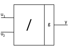
Figure 11.2.2 Finite Element Cross Section

11.2.4.2. Incremental Form of the Virtual Work Equations

Eq. (11.2-65) can be viewed as expressing the balance between the external forces on the right hand side and the internal forces on the left hand side. The external forces are known functions of time. The stress field on the other hand must be found to satisfy the Eq. (11.2-65) and the constitutive laws for the material. Since the constitutive equations are, in general, highly non-linear, an incremental technique is used in FPIN2 based on iterations within each increment to calculate the stresses.

Assuming that all the stresses at time $t_{\text{i}}$ are known, the equilibrium equation, Eq. (11.2-65), can be rewritten at the end of the time step, $t_{\text{i}+1}$, as

(11.2-68) $$\underline{\Delta f}^{\text{int}} = \underline{\Delta f}^{\text{ext}}$$

where

(11.2-69) $$\underline{\Delta f}^{\text{int}} = \underline{f}_{\text{i} + 1}^{\text{int}} - \underline{f}_{\text{i}}^{\text{int}} = \int_{\text{A}_{\text{e}}} \left\lbrack B \right\rbrack^{T} \underline{\Delta \sigma} \text{dA}$$

and

(11.2-70) $$\underline{\Delta f}^{\text{ext}} = \underline{f}_{\text{i} + 1}^{\text{ext}} - \underline{f}_{\text{i}}^{\text{ext}}$$

The problem has now been reduced to finding the stress increments $\underline{\Delta \sigma}$ appearing implicitly in Eq. (11.2-68) through Eq. (11.2-69). These stress increments

(11.2-71) $$\underline{\Delta \sigma} = \underline{\sigma}_{\text{i} + 1} - \underline{\sigma}_{\text{i}}$$

are calculated through an iterative procedure.

As discussed in Section 11.2.1.5, the stress increments are approximated by Eq. (11.2-27) that is repeated here

(11.2-72) $$\underline{\Delta \sigma} = \left\lbrack C \right\rbrack_{\text{i}} \underline{\Delta \varepsilon}^{a} - \underline{\Delta \sigma}_{\text{i}}^{\text{ps}}$$

where the elastic modulus, $\left\lbrack C \right\rbrack_{\text{i}}$, and pseudo-stress, ${\underline{\Delta \sigma}^{\text{ps}}}_{\text{i}}$, are evaluated using values at $t_{\text{i}}$ (or at $t_{\text{i}+1}$ if known). The apparent strain increment, $\underline{\Delta \varepsilon}^{a}$, in Eq. (11.2-72) can be expressed in terms of displacement increments through the strain-displacement relations, as discussed in Section 11.2.1.1. Using a similar representation with the virtual work functions, $\phi_{\text{r}}$ and $\phi_{\text{z}}$, radial and axial displacement increments can be written as

(11.2-73) $$\Delta u = \Delta u_{1} N_{1} + \Delta u_{2} N_{2}$$

(11.2-74) $$\Delta w = z\Delta\psi$$

Using these in Eq. (11.2-8) leads to

(11.2-75) $$\underline{\Delta \varepsilon}^{a} = \left\lbrack B \right\rbrack \underline{\Delta \delta}$$

where

(11.2-76) $$\underline{\Delta \delta} = \left\{ \Delta u_{1}, \Delta u_{2}, \Delta\psi \right\}^{T}$$

After substituting Eq. (11.2-75) into Eq. (11.2-72), and subsequently replacing the result in Eq. (11.2-69), we can rewrite the equilibrium equation, E. Eq. (11.2-68), in the form

(11.2-77) $$\left\lbrack K \right\rbrack_{\text{i}} \underline{\Delta \delta} = \underline{f}^{\text{ext}} + \underline{f}_{\text{i}}^{\text{ps}}$$

where

(11.2-78) $$\left\lbrack K \right\rbrack_{\text{i}} = \int_{\text{A}_{\text{e}}}{\left\lbrack B \right\rbrack_{\text{i}}^{T} \left\lbrack C \right\rbrack_{\text{i}}} \left\lbrack B \right\rbrack_{\text{i}}\text{dA}$$

and

(11.2-79) $$\underline{\Delta f}_{\text{i}}^{\text{ps}} = \int_{\text{A}_{\text{e}}}{\left\lbrack B \right\rbrack_{\text{i}}^{T} \underline{\Delta \sigma}_{\text{i}}^{\text{ps}}\text{dA}}$$

Here $\left\lbrack K \right\rbrack_{\text{i}}$ is the stiffness matrix evaluated at $t_{\text{i}}$ using the known values. It should be noted that the forms of the matrices $\left\lbrack C \right\rbrack$ and $\left\lbrack B \right\rbrack$ in Eq. (11.2-78) and $\underline{\Delta \sigma}^{\text{ps}}$ in Eq. (11.2-70) depend on the type of element considered as discussed earlier in Section 11.2.1.5. Explicit formulas for the stiffness matrix and load vectors for both element types considered are given in Section 11.7.1.

11.2.4.3. Iterative Solution of the Equilibrium Equations

Eq. (11.2-77) is the incremental form of the virtual work (or equilibrium) equation. Since the stiffness matrix $\left\lbrack K \right\rbrack_{\text{i}}$ is known, it constitutes a set of linear equations that can be solved for the displacement increments, $\underline{\Delta \delta}$. Eq. (11.2-75) then gives the increment in apparent total strain, $\underline{\Delta \varepsilon}$, and the algorithm described in Section 11.2.2 gives the stresses at time $t_{\text{i}+1}$. These stresses, in turn, can be used in Eq. (11.2-69) to calculate the internal force vector. However, since the expression for the stress increment in Eq. (11.2-72) is only approximate, the equilibrium equation Eq. (11.2-68) will not be satisfied in general.

In FPIN2, another iterative procedure is used to ensure that the stress estimates satisfy the equilibrium equation to an acceptable degree of accuracy. By defining the residual, or the error, in Eq. (11.2-68) as follows

(11.2-80) $$\underline{r} = \underline{f}_{\text{i} + 1}^{\text{ext}} - \underline{f}_{\text{i} + 1}^{\text{int}}$$

The successive evaluations of the nodal variable increments, $\underline{\Delta \delta}$, are calculated from

(11.2-81) $$\left( K \right)_{\text{i}}\underline{\Delta \delta}_{\text{j}} = \underline{\Delta f}^{\text{ext}} + \underline{\Delta f}_{\text{i}}^{\text{ps}} + \underline{r}_{\text{j} - 1}$$

where $j$ is the iteration index.

The convergence of this iterative scheme is monitored through the norm of the residual vector. If this error is sufficiently small, then the equilibrium equations are assumed to be satisfied and the computation is advanced to the next time step. Otherwise, the new residual vector $\underline{r}_{\text{j}}$, is calculated and added to the right hand side of Eq. (11.2-81) (the previous residual vector, $\underline{r}_{\text{i} + 1}$, remains there as well). Figure 11.2.3 summarizes this algorithm for iterative solution of the equilibrium equations.

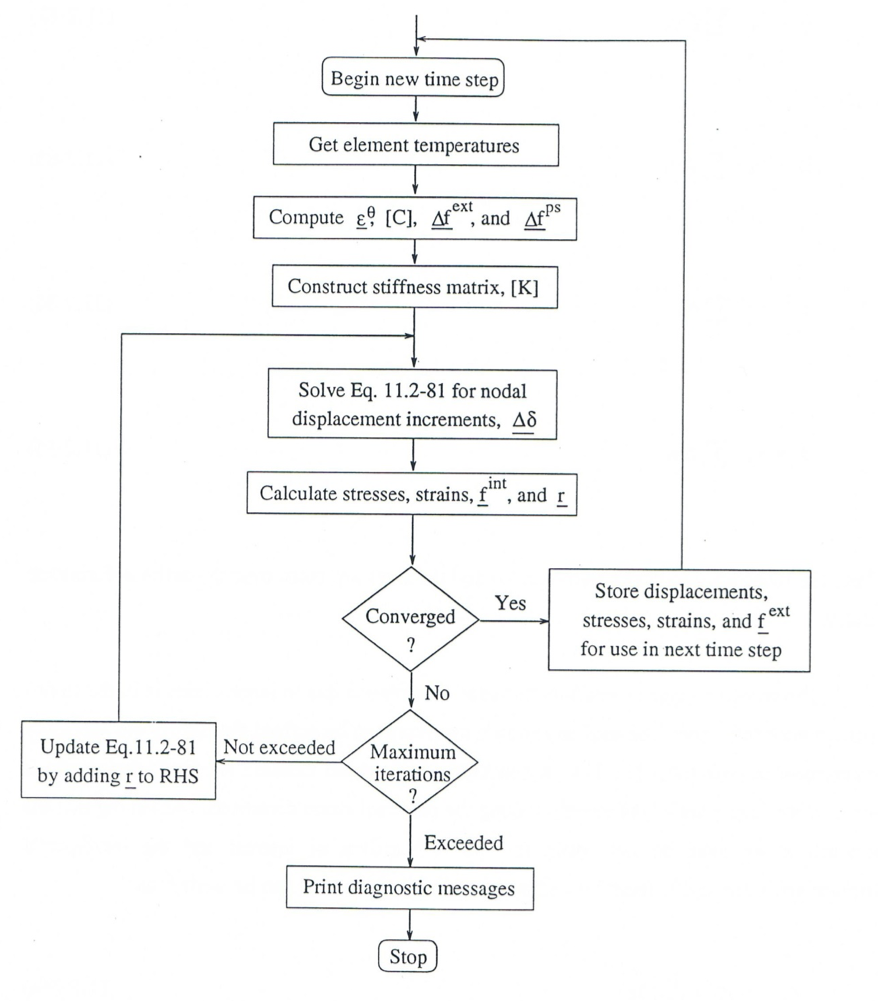
Figure 11.2.3 Iterative Solution of Equilibrium Equations

11.2.5. Large Strain Analysis

Since fuel pin deformation at high temperatures may involve large plastic strains as well as massive local swelling, it is important that the formation of the mechanics model allows for analysis of large strains. Consideration of large strains has impacts on the equilibrium equations derived in Section 11.2.4 and the strain-displacement definitions given in Section 11.2.1. Both changes involve straightforward modifications of the incremental (small perturbation) analysis that has already been derived.

Since the stresses at any time $t_{\text{i}+1}$ must satisfy the equilibrium equations Eq. (11.2-57) in the deformed cylindrical geometry, the virtual work equations should be applied to the fuel element geometry at $t_{\text{i}+1}$ rather than the initial geometry as assumed previously. Following through the derivation of the finite-element equilibrium equation, Eq. (11.2-65), it is easy to show that the only change necessary to accommodate large strains is to redefine the geometric variables to refer to the deformed element. Furthermore, if the incremental deformation between times $t_{\text{i}}$ and $t_{\text{i}+1}$ is small, negligible error will be incurred by replacing the geometric variables at $t_{\text{i}+1}$ by these values at $t_{\text{i}}$. These values are readily available form the initial undeformed geometry and the known deformation. From Eq. (11.2-73) and Eq. (11.2-74) for instance, we have

(11.2-82) $$a = a_{0} + \sum_{\text{i}}{\Delta u_{1}}$$

(11.2-83) $$b = b_{0} + \sum_{\text{i}}{\Delta u_{2}}$$

(11.2-84) $$r = r_{0} + \sum_{\text{i}}{\Delta u}$$

(11.2-85) $$z = z_{0} + \sum_{\text{i}}{\Delta w}$$

where the subscript 0 indicates the initial values, and the sums are taken over the entire deformation history.

The second change in small-perturbation formulation due to large strains is in the strain-displacement definitions. Several large strain measures can be defined that satisfy the necessary requirement of objectivity [11-11]. A convenient large strain measure for the fuel elements is given by the logarithm of the stretches along the principal strain directions. Assuming that the principal strain axes do not rotate for the deformation of interest and the incremental displacements are small, these logarithmic large strain measures can be written as

(11.2-86) $$\varepsilon_{\text{r,i} + 1}^{t} = \varepsilon_{\text{r,i}}^{t} + \frac{\partial}{\partial \text{r}_{\text{i}}} \left( \Delta u \right)$$

(11.2-87) $$\varepsilon_{\theta,\text{i} + 1}^{t} = \varepsilon_{\theta,\text{i}}^{t} + \frac{\Delta u}{r_{\text{i}}}$$

(11.2-88) $$\varepsilon_{\text{z,i} + 1}^{t} = \varepsilon_{\text{z,i}}^{t} + \frac{\partial}{\partial \text{z}_{\text{i}}} \left( \Delta w \right)$$

Comparing Eq. (11.2-86) with Eq. (11.2-5) shows that, in order to use the logarithmic large strain measure, the only change necessary in the analysis given previously is to use the displacement increments to calculate the strain increments and then to determine total strains by adding the increments throughout the deformation history.

Footnotes

[4]

If the fuel-cladding gap is closed, this resultant axial force may include both fuel and cladding.

[5]

Because of the definition of crack strain in Eq. (11.2-7), ${}^{c}$ will be negative for opening of cracks. The crack strain input to and output from FPIN2 is the absolute value of this quantity.

[6]

To define $\phi_{r}$ over the entire domain of the integration, $A$, we must cover the domain with a finite element mesh and then sum the contributions at each node from all elements sharing the node. For brevity, this finite element assembly process is not discussed here and formulation is developed for a single element only.