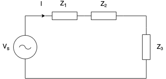
5.16.7. Appendix 5.7: Detailed Derivation of EQ EM Pump

The equivalent circuits for the detailed and the simple EM pump models can be reduced to the circuit shown in Figure 5.16.2, where $Z_{i}$ is the impedance of each component in the path of the total phase current, $I$, being driven by the phase voltage, $V_{s}$.

Figure 5.16.2 Reduced Equivalent Circuit for the EM pump models.

Because the equivalent circuits contain inductors, the circuit’s total impedance is a complex number.

(5.16-71) $$\begin{split}Z_{T} &= Z_{1} + Z_{2} + Z_{3} \\ &= Re\left( Z_{T} \right) + Im(Z_{T})j \\ &= Re\left( Z_{1} \right) + Re\left( Z_{2} \right) + Re\left( Z_{3} \right) + Im\left( Z_{1} \right)j + Im\left( Z_{2} \right)j + Im\left( Z_{3} \right)j\end{split}$$

Using the total impedance, the total phase current can be quantified using Ohm’s law.

(5.16-72) $$\begin{split}I &= \frac{V}{Z_{T}} \\ |I| &= \frac{|V|}{{|Z}_{T}|} \\ |I| &= \frac{|V|}{\sqrt{\text{Re}\left( Z_{T} \right)^{2} + Im\left( Z_{T} \right)^{2}}}\end{split}$$

The presence of the inductors introduces a phase difference between the phase voltage and current. The phase difference is defined as

(5.16-73) $$\tan\left( \phi \right) = \frac{\text{Im}\left( Z_{T} \right)}{Re(Z_{T})}$$

5.16.7.1. Simple Circuit Analysis

For the simple EM pump circuit, the impedance of each component is

(5.16-74) $$Z_{1} = R_{1}$$

(5.16-75) $$Z_{2} = X_{1}j$$

(5.16-76) $$Z_{3} = \left( \frac{1}{X_{2}j} + \frac{s}{R_{2}} \right)^{- 1} = \frac{R_{2}X_{2}j}{R_{2} + \text{sX}_{2}j} = \frac{sR_{2}X_{2}^{2}}{R_{2}^{2} + s^{2}X_{2}^{2}} + \frac{R_{2}^{2}X_{2}}{R_{2}^{2} + s^{2}X_{2}^{2}}j$$

Using Eq. (5.16-71) and Eq. (5.16-72), the current as a function of slip, frequency and voltage can be determined.

(5.16-77) $$|I| = \frac{|V|}{\sqrt{\left( R_{1} + \frac{sR_{2}X_{2}^{2}}{R_{2}^{2} + s^{2}X_{2}^{2}} \right)^{2} + \left( X_{1} + \frac{R_{2}^{2}X_{2}}{R_{2}^{2} + s^{2}X_{2}^{2}} \right)^{2}}}$$

The current’s dependence on slip is inherent, as $X_{i} = 2\pi L_{i} f$.

Ohm’s law can be used to determine the division of the total current between the $X_{2}$ and $R_{2}/s$ branches

(5.16-78) $$\left| I \right|\left| Z_{3} \right| = \left| I_{1} \right|\left| X_{2} \right| = \left| I_{2} \right|\frac{R_{2}}{s}$$

Therefore, the power dissipated in $R_{2}/s$ can be defined as

(5.16-79) $$\begin{split}P_{R2} &= 3\left| I_{2} \right|\left| V_{R2} \right| \\ &= 3\frac{\left| I_{2} \right|^{2}R_{2}}{s}\end{split}$$

If we assume that a fraction of the power is lost to the fluid, the mechanical power dissipated in $R_{2}/s$ is

(5.16-80) $$\begin{split}P_{R2} &= 3\frac{\left| I_{2} \right|^{2}R_{2}\left( 1 - s \right)}{s} \\ &= 3\left| I \right|^{2}\left| Z_{3} \right|^{2}\left( 1 - s \right)\frac{R_{2}}{s} \\ &= 3\left| I \right|^{2}\left( \frac{\left| Z_{3} \right|}{\frac{R_{2}}{s}} \right)^{2}\left( 1 - s \right)\frac{R_{2}}{s} \\ &= 3\frac{s^{4}X_{2}^{4} + {s^{2}R}_{2}^{2}X_{2}^{2}}{\left( R_{2}^{2} + s^{2}X_{2}^{2} \right)^{2}}\left( 1 - s \right)\frac{R_{2}}{s}\left| I \right|^{2} \\ &= 3\frac{s^{2}X_{2}^{2}}{\left( R_{2}^{2} + s^{2}X_{2}^{2} \right)}\left( 1 - s \right)\frac{R_{2}}{s}\left| I \right|^{2} \\ &= 3\left| I \right|^{2}\frac{R_{2}(1 - s)}{\text{s}\left( \frac{R_{2}^{2}}{s^{2}X_{2}^{2}} + 1 \right)}\end{split}$$

Using the relationship between pumping power and pump head, the developed pump head for the simple EM pump model can be described as

(5.16-81) $$\begin{split}\Delta P_{\text{pump}} &= \frac{P_{R2}}{Q} \\ &= 3\left| I \right|^{2}\frac{R_{2}(1 - s)}{\text{Qs}\left( \frac{R_{2}^{2}}{s^{2}X_{2}^{2}} + 1 \right)}\end{split}$$

5.16.7.2. Detailed Circuit Analysis

For the detailed EM pump circuit, the impedance of each component is

(5.16-82) $$Z_{1} = R_{1}$$

(5.16-83) $$Z_{2} = X_{1}j$$

(5.16-84) $$\begin{split}Z_{3} &= \left( \frac{1}{X_{2}j} + \frac{1}{R_{D}} + \frac{1}{R_{J} + R_{m}} \right)^{- 1} \\ &= \frac{\left( R_{J} + R_{M} \right)R_{D}X_{2}j}{\left( R_{J} + R_{m} \right)R_{D} + \left( R_{J} + R_{M} + R_{D} \right)X_{2}j} \\ &= \frac{\left( R_{J} + R_{m} \right)\left( R_{J} + R_{m} + R_{D} \right)R_{D}X_{2}^{2} + \left( R_{J} + R_{m} \right)^{2}R_{D}^{2}X_{2}j}{\left( R_{J} + R_{m} \right)^{2}R_{D}^{2} + \left( R_{J} + R_{m} + R_{D} \right)^{2}X_{2}^{2}}\end{split}$$

The magnitude of $Z_{3}$ is

(5.16-85) $$\begin{split}\left| Z_{3} \right|^{2} &= \frac{\left( R_{J} + R_{m} \right)^{2}\left( R_{J} + R_{m} + R_{D} \right)^{2}R_{D}^{2}X_{2}^{4} + \left( R_{J} + R_{m} \right)^{4}R_{D}^{4}X_{2}^{2}}{\left( \left( R_{J} + R_{m} \right)^{2}R_{D}^{2} + \left( R_{J} + R_{m} + R_{D} \right)^{2}X_{2}^{2} \right)^{2}} \\ &= \frac{\left( R_{J} + R_{m} \right)^{2}R_{D}^{2}X_{2}^{2}}{\left( R_{J} + R_{m} \right)^{2}R_{D}^{2} + \left( R_{J} + R_{m} + R_{D} \right)^{2}X_{2}^{2}}\end{split}$$

Using a similar analysis as was presented for the simple model, the current passing through the fluid is determined to be

(5.16-86) $$\left| I \right|\left| Z_{3} \right| = \left| I_{3} \right|(R_{J} + R_{m})$$

and the mechanical power delivered to the fluid is

(5.16-87) $$\begin{split}P_{m} &= 3\left| I_{3} \right|^{2}R_{m} \\ &= 3\frac{\left| I \right|^{2}\left| Z_{3} \right|^{2}}{\left( R_{J} + R_{m} \right)^{2}}R_{m} \\ &= 3I^{2}R_{m}\frac{R_{D}^{2}X_{2}^{2}}{\left( R_{J} + R_{m} \right)^{2}R_{D}^{2} + \left( R_{J} + R_{m} + R_{D} \right)^{2}X_{2}^{2}}\end{split}$$

Therefore, the developed pump head in the detailed EM pump model is

(5.16-88) $$\begin{split}\Delta P &= \frac{P_{m}}{Q} \\ &= 3 \frac{I^{2}R_{m}}{Q}\frac{R_{D}^{2}X_{2}^{2}}{\left( R_{J} + R_{m} \right)^{2}R_{D}^{2} + \left( R_{J} + R_{m} + R_{D} \right)^{2}X_{2}^{2}}\end{split}$$

5.16.7.3. Simple Circuit Parameters

In order to determine the resistance and inductance of the different components in the simple EM pump model, measurable quantities are provided at two distinct pump states. The first pump state, referred to as the rated state, provides a pump head, $\Delta P_{R}$, measured flow rate, $Q_{R}$, measured phase voltage, $V_{R}$, measured phase current, $I_{R}$, measured slip, $s_{R}$, measured efficiency, $\eta_{R}$, and measured frequency, $f_{R}$. The second pump state, referred to as the stalled state, provides the pump head at stalled conditions, $\Delta P_{S}$, for the measured frequency and measured phase voltage. $\Delta P_{P,R}$ and $\Delta P_{S,R}$ are functions of the measured pump head, $\Delta P_{R}$, and measured pump head at stalled conditions, $\Delta P_S$.

When IDPOPT = 0, then the user-provided $\Delta P_{R}$ and $\Delta P_{S}$ include pressure changes due to friction losses across the pump. When IDPOPT = 1, then the user-provided $\Delta P_{R}$ and $\Delta P_{S}$ do not include pressure changes due to friction losses across the pump.

To solve the initial conditions for the simplified pump model, the following terms are defined.

(5.16-89) $$\Delta P_{P,S} = \Delta P_{S}$$

$$\begin{split}\Delta P_{P,R} = \begin{cases} \begin{aligned} &\Delta P_R, & \text{IDPOPT} &\neq 0 \\ &\Delta P_R + \Delta P_{f,R}, & \text{IDPOPT} &= 0 \end{aligned} \end{cases}\end{split}$$

where $\Delta P_{f,R}$ is the frictional pressure drop that occurs within the pump at the rated flow rate and IDPOPT is a user-defined flag. $\Delta P_{f,R}$ is internally calculated by SAS4A/SASSYS‑1 using the geometry input.

In order to determine the 4 circuit parameters and the current at stalled conditions, five equations are required. Ohm’s law provides us with two of the five equations:

(5.16-90) $$\left( \frac{V_{R}}{I_{R}} \right)^{2} = \left| Z_{T}(s = s_{R}) \right|^{2}$$

(5.16-91) $$\left( \frac{V_{R}}{I_{S}} \right)^{2} = \left| Z_{T}(s = 1) \right|^{2}$$

The rated and stall pressures provide an additional two equations:

(5.16-92) $$\Delta P_{P,R} = \frac{3I_{R}^{2}R_{2}}{Av_{s}\left( \frac{R_{2}^{2}}{X_{2}^{2}s_{R}} + s_{R} \right)}$$

(5.16-93) $$\Delta P_{P,S} = \frac{3I_{s}^{2}R_{2}}{Av_{s}\left( \frac{R_{2}^{2}}{X_{2}^{2}} + 1 \right)}$$

The final equation comes from the total power dissipated by the pump

(5.16-94) $$P_{R} = 3V_{R}I_{R}\cos\left( \phi \right)$$

(5.16-95) $$\cos\left( \phi \right) = \frac{\text{Re}\left( Z_{T}\left( s = s_{R} \right) \right)}{|Z_{T}\left( s = s_{R} \right)|}$$

(5.16-96) $$P_{R} = \frac{\left( \Delta P_{R} \right)Q_{R}}{\eta_{R}}$$

(5.16-97) $$Re\left(Z_T(s=s_R)\right)^2 = \left(\frac{\left( \Delta P_{R} \right)Q_{R}}{3I_R^2\eta_{R}}\right)^2$$

Note, the synchronous speed of the EM pump can be determined using the definition of slip and the rated conditions

(5.16-98) $$v_{s}A = \frac{Q_{R}}{1 - s_{R}}$$

Instead of solving the five equations at once, an iterative approach is taken. By assuming a stall current, Eq. (5.16-93) can be solved

(5.16-99) $$\frac{R_{2}^{2}}{X_{2}^{2}} = \frac{3I_{s}^{2}R_{2}}{Av_{s}\Delta P_{s}} - 1$$

and plugged into Eq. (5.16-92), providing an equation for $R_{2}$

(5.16-100) $$R_{2} = \frac{\left( \Delta P_{P,R} \right)\left( Av_{s}\frac{\left( s_{R}^{2} - 1 \right)}{s_{R}} \right)}{3I_{R}^{2} - \frac{3I_{S}^{2}}{\Delta P_{P,S}s_{R}}\Delta P_{P,R}}$$

with the value of $R_{2}$ known, $X_{2}$ can be determined using Eq. (5.16-99) and Eq. (5.16-97) can be solved to determine the value of $R_{1}$

(5.16-101) $$R_{1} = \frac{\left( \frac{{\Delta P}_{R}Q_{R}}{3I_{R}^{2}\eta_{R}}\left( R_{2}^{2} + X_{2}^{2}{s_{R}}^{2} \right) - s_{R}R_{2}X_{2}^{2} \right)}{\left( R_{2}^{2} + X_{2}^{2}s_{R}^{2} \right)}$$

With $R_{1}$, $R_{2}$, and $X_{2}$ known Eq. (5.16-90) can be used to determine $X_{1}$

(5.16-102) $$X_{1} = \left\lbrack \left( \frac{V_{R}}{I_{R}} \right)^{2} - \text{Re}\left( Z_{T}(s = s_{R}) \right)^{2} \right\rbrack^{1/2} - \frac{R_{2}^{2}X_{2}}{\left( R_{2}^{2} + X_{2}^{2}s_{R}^{2} \right)}$$

Finally, Eq. (5.16-91) will be solved to determine the error in the stall current. Using error in the stall current, a new stall current will be estimated and Eq. (5.16-99) through Eq. (5.16-102) will be repeated. This process continues until the error in the stall current is within a user defined limit.