3.19. Appendices

3.19.1. APPENDIX 3.1: Degree of Implicitness for Flow and Temperature Calculations

A typical calculation in SASSYS-1 involves finding a temperature or flow rate at the end of a time step given the values of relevant parameters at the beginning of the step, as well as the values of driving functions at the beginning and end of the step. Linearized finite difference approximations to the relevant differential equations are usually used, and the accuracy of the finite differencing in time will depend both on the size of the time step and on the degree of implicitness in the solution. By picking appropriate values for the degree of implicitness, it is possible to improve the accuracy of the solution.

The differential equations used for temperatures and flow rates are of the form

(A3.1‑1)

\[\frac{\text{dy}}{\text{dt}} = f\left( y,t \right)\]

Where \(y\) is the flow rate or temperature being calculated, and \(f\) is a function of y and time. The finite difference approximation used for Eq. A3.1-1 is

(A3.1‑2)

\[\frac{y_{2} - y_{1}}{ \Delta t } = \theta_{1}f\left( y_{1},t_{1} \right) + \theta_{2}f\left( y_{2},t_{2} \right)\]

where

\(t_1\) = time at the beginning of the time step

\(t_2\) = time at the end of the time step

\(y_1\) = \(y\) at \(t_1\)

\(y_2\) = \(y\) at \(t_2\)

(A3.1‑3)

\[\Delta t = t_{2} - t_{1}\]

(A3.1‑4)

\[\theta_{1} + \theta_{2} = 1.0\]

The parameters \(\theta_1\) and \(\theta_2\) determines the degree of implicitness of the solution: for a fully explicit solution \(\theta_1\) = 1.0 and \(\theta_2\) = 0.0, whereas for a fully implicit solution \(\theta_1\) = 0.0 and \(\theta_2\) = 1.0.

After linearizing, equation A3.1-1 can be put in the form

(A3.1‑5)

\[\frac{\text{dy}}{\text{dt}} = f\left( y_{1},t_{1} \right) + \left( t - t_{1} \right)\frac{\text{df}}{\text{dt}} + \left( y - y_{1} \right)\frac{\text{df}}{\text{dy}}\]

or

(A3.1‑6)

\[\frac{\text{dy}}{\text{dt}} = A + B \left( t - t_{1} \right) + C\left( y - y_{1} \right)\]

where

(A3.1‑7)

\[A = f\left( y_{1},t_{1} \right)\]

(A3.1‑8)

\[B = \frac{\text{df}}{\text{dt}}\]

(A3.1‑9)

\[C = \frac{\text{df}}{\text{dy}}\]

For instance Eq. (3.9-8) for the coolant flow rate in a channel is

(A3.1‑10)

\[I_{1}\frac{\text{dw}}{\text{dt}} = p_{\text{b}} - p_{\text{t}} - w^{2}I_{2} - A'_{\text{fL}}wI_{\text{3L}} - A'_{\text{fr}}w \left| w \right|^{1 + b_{\text{fr}}}I_{\text{3T}} - w\left| w \right|I_{4} - gI_{5}\]

Linearizing the \(w^2\), \(w \left| w \right|^{1 + b_{\text{fr}}}\), and \(w\left| w \right|\) terms gives

(A3.1‑11)

\[w^{2} \simeq w_{1}^{2} + 2w_{1}\left( w - w_{1} \right)\]

(A3.1‑12)

\[w \left| w \right|^{1 + b_{\text{fr}}} \simeq w_{1}\left| w_{1} \right|^{1 + b_{\text{fr}}} + \left( 2 + b_{\text{fr}} \right) \left| w_{1} \right|^{1 + b_{\text{fr}}}\left( w - w_{1} \right)\]

and

(A3.1‑13)

\[w \left| w \right| \simeq w_{1}\left| w_{1} \right| + \left| w_{1} \right|\left( w - w_{1} \right)\]

Also, \(p_{\text{b}}\) and \(p_{\text{t}}\) are approximated as

(A3.1‑14)

\[p_{\text{b}}\left( t \right) = p_{\text{b}}\left( t_{1} \right) + \left( t - t_{1} \right)\frac{\text{dp}_{\text{b}}}{\text{dt}}\]

(A3.1‑15)

\[p_{\text{t}}\left( t \right) = p_{\text{t}}\left( t_{1} \right) + \left( t - t_{1} \right)\frac{\text{dp}_{\text{t}}}{\text{dt}}\]

where

(A3.1‑16)

\[\frac{\text{dp}_{\text{b}}}{\text{dt}} = \frac{p_{\text{b}}\left( t_{2} \right) - p_{\text{b}}\left( t_{1} \right)}{t_{2} - t_{1}}\]

and

(A3.1‑17)

\[\frac{\text{dp}_{\text{t}}}{\text{dt}} = \frac{p_{\text{t}}\left( t_{2} \right) - p_{\text{t}}\left( t_{1} \right)}{t_{2} - t_{1}}\]

Then Eq. A3.1-10 has the form of A3.1-16 if

(A3.1‑18)

\[A = \frac{\left\{ p_{\text{b}}\left( t_{1} \right) - p_{\text{t}}\left( t_{1} \right) - w_{1}^{2}I_{2} - A'_{\text{fL}}w_{1}I_{\text{3L}} - A'_{\text{fr}} w_{1}\left| w_{1} \right|^{1 + b_{\text{fr}}} I_{\text{3T}} - w_{1} \left| w_{1} \right|\ I_{4} - gI_{5} \right\}}{I_{1}}\]

(A3.1‑19)

\[B = \frac{\frac{\text{dp}_{\text{b}}}{\text{dt}} - \frac{\text{dp}_{\text{t}}}{\text{dt}}}{I_{1}}\]

and

(A3.1‑20)

\[C = - \frac{\left\lbrack 2w_{1} I_{2} - A'_{\text{fL}}I_{\text{3L}} - \left( 2 + b_{\text{fr}} \right)A'_{\text{fr}}\left| w_{1} \right|^{1 + b_{\text{fr}}}I_{\text{3T}} - \left| w_{1} \right|I_{4} \right\rbrack}{I_{1}}\]

The exact solution for Eq. A3.1-6 is

(A3.1‑21)

\[y - y_{1} = \left( A\tau - B\tau^{2} \right) \left( 1 - e^{- \left( t - t_{1} \right)/\tau} \right) + B\tau\left( t - t_{1} \right)\]

where

(A3.1‑22)

\[\tau = - \frac{1}{C}\]

The finite difference approximation used for Eq. A3.1-6 is

(A3.1‑23)

\[\frac{y_{2} - y_{1}}{ \Delta t } = A + \theta_{2}B\Delta t + \theta_{2} C \left( y_{2} - y_{1} \right)\]

where

(A3.1‑24)

\[\Delta t = t_{2} - t_{1}\]

The solution of Eq. A3.1-23 for \(y_2\) is

(A3.1‑25)

\[y_{2} - y_{1} = \frac{\Delta t + \theta_{2} B\Delta t^{2}}{1 + \theta_{2} \frac{\Delta t}{\tau}}\]

Figure 3.19.1 shows \(y_2\) - \(y_1\), as given by Eq. A3.1-25, as a function of \(\theta_2\) for the case where \(A\) = 1, \(B\) = .5, \(\Delta t\) = 2, and \(\tau\) = 1. Also shown is the exact solution from Eq. A3.1-21. Note that a value \(\theta_2\) can be found such that the finite difference solution of Eq. A3.1-25 exactly matches the differential equation solution, given by Eq. A3.1-21, for this case. Also note that neither a fully explicit solution, \(\theta_2\) = 0, nor a fully implicit solution, \(\theta_2\) = 1.0, is very accurate for particular case. An explicit solution would be numerically unstable for \(\Delta t\) greater than \(\tau\); and values considerably smaller than the time constant \(\tau\).

For any values of the parameters in Eq. A3.1-21 and Eq. A3.1-25, a value of \(\theta_2\) can be chosen such that the finite difference solution matches the solution of the differential equation by setting \(t = t_2\) in Eq. A3.1-21 and combining this equation with Eq. A3.1-25 to give

(A3.1‑26)

\[\left( A\tau - B\tau^{2} \right) \left( 1 - e^{- \Delta t/\tau} \right) + B \tau \Delta t = \frac{\Delta t + \theta_{2} B\Delta t^{2}}{1 + \theta_{2} \frac{\Delta t}{\tau}}\]

solving for \(\theta_2\) gives

(A3.1‑27)

\[\theta_{2} = \frac{\frac{ \Delta t }{\tau} - \left( 1 - e^{- \Delta t/\tau} \right)}{\frac{ \Delta t }{\tau}\left( 1 - e^{- \Delta t/\tau} \right)}\]

Note that A and B cancelled out of Eq. A3.1-27, and \(\theta_2\) is a function only of \(\Delta t/t\).

Figure 3.19.2 shows \(\theta_2\), given by Eq. A3.1-27, as a function of \(\Delta t/\tau\). This figure also shows some approximations to this function, as discussed below. For small values of \(\Delta t/\tau\), \(\theta_2\) approaches 0.5, where as for large values of \(\Delta t/\tau\), \(\theta_2\) approaches 1.0.

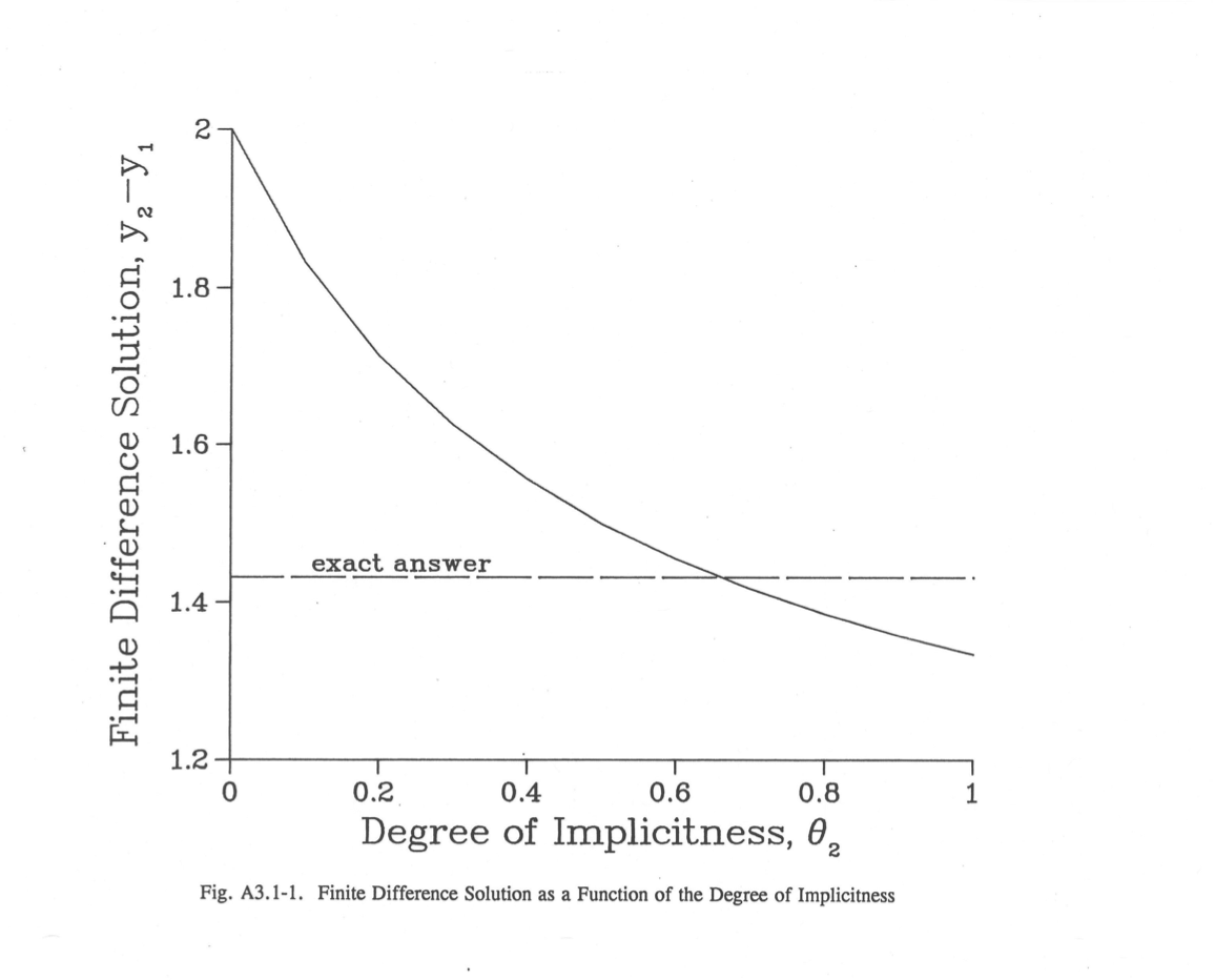
Figure 3.19.1 Finite Difference Solution as a Function of the Degree of Implicitness

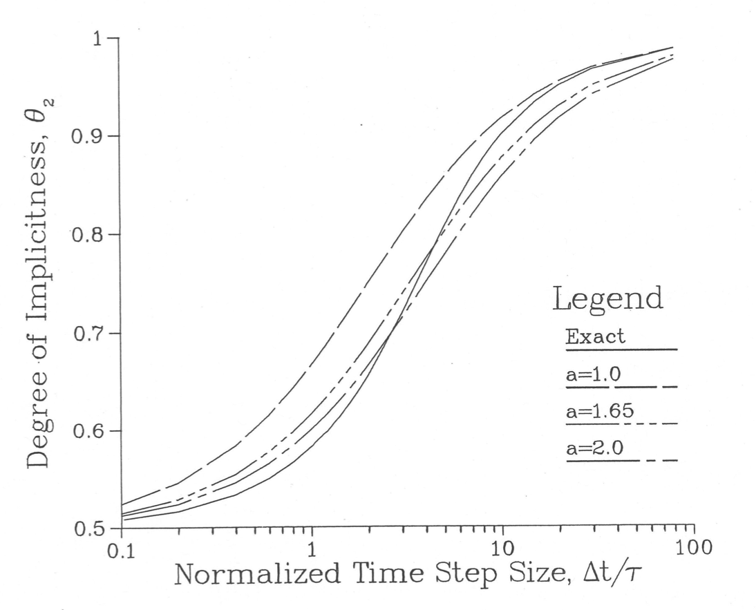
Figure 3.19.2 Degree of Implicitness as a Function of Normalized Time Step Size

For any equation that can be put in the form of Eq. A3.1-5 or A3.1-6, Eq. A3.1-22 can be used to find \(\tau\), and then Eq. A3.1-27 can be used to find the appropriate value of \(\theta_2\) for any value of \(\Delta t\). Note that if driving pressures and coolant flows are being solved for simultaneously, as is done in PRIMAR-4, then the value of \(B\) in Eq. A3.1-6 is not known until the pressures have been solved for. In such cases, a direct analytic solution of the differential equation, as in Eq. A3.1-22, could not be made except by iterating between Eq. A3.1-22 and the pressure solution. On the other hand, the calculation of \(\theta_2\), as in Eq. A3.1-27, requires only \(\Delta t\) and \(\tau\); and the calculation of \(\tau\) requires only information that is available at the beginning of a time step; so an appropriate value for \(\theta_2\) can be found for use in finite difference approximations without iteration, even if driving pressures and flow rates are being solved for simultaneously.

Even if finite differencing in time does not introduce any error into a solution, there are usually other sources of error, such as the linearization approximations of Eq. A3.1-11 through Eq. A3.1-17. Also, the term represented by \(B \left(t-t_1 \right)\) in Eq. A3.1-6 may in fact not be linear in time. Therefore, simpler and easier to compute approximations to the expression on the right-hand side of Eq. A3.1-27 might sometimes be used without losing much overall accuracy. A simple approximation, \({\theta'}_{2}\) that approaches the correct limits for very small and very large values of \(\Delta t/\tau\) is

(A3.1‑28)

\[{\theta'}_{2} = \frac{a + \frac{ \Delta t }{\tau}}{2a + \frac{ \Delta t }{\tau}}\]

where the parameter \(a\) can be chosen to give some best overall fit. Figure 3.19.2 shows this function for various values of the parameter \(a\). The curve for \(a\) = 1.65 gives a fairly good fit, although no value of \(a\) will give a good fit over the whole range.

A better fit to \(\theta_2\) can be obtained by an expression of the form

(A3.1‑29)

\[{\theta'}_{2} = \frac{a + bx + x^{2}}{2a + cx + x^{2}}\]

where

(A3.1‑30)

\[x = \frac{ \Delta t }{\tau}\]

with \(a\) = 6.12992, \(b\) = 2.66054, and \(c\) = 3.56284, this expression fits the exact value of Eq. A3.1-27 to within 1% over the whole range of \(\Delta t/\tau\), as shown in Figure 3.19.3.

In general, when linear approximations are valid, and when a single known time constant dominates the behavior, Eq. A3.1-27 or Eq. A3.1-29 will give a value of \(\theta_2\) that will provide accurate finite difference solutions. For cases where a number of different time constants are important, none of these expressions for \(\theta_2\) will give a precise finite difference solution for all time-step sizes. Even in this case, though, \(\theta_2\) should approach 0.5 for small time steps, and it should approach 1.0 for large time steps. Therefore, an expression of the form given by Eq. A3.1-28 may be appropriate in such cases.

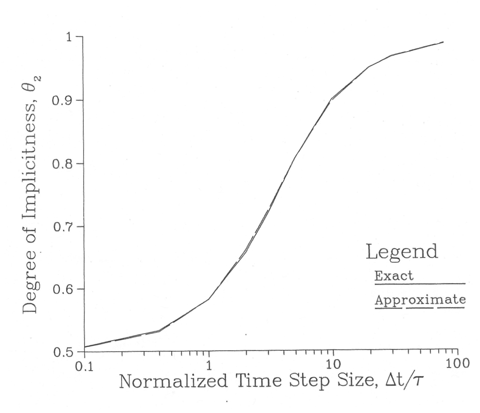
Figure 3.19.3 Approximate Correlation for the Degree of Implicitness

3.19.2. APPENDIX 3.2: Input Preprocessor

3.19.2.1. Introduction

A preliminary version of an input preprocessor has been written for the three-dimensional core thermal hydraulics model described in Section 3.14. This preprocessor reads a relatively small amount of information from the user and produces a large fraction of the input for the new model. This appendix is split into two main sections. The first section details the calculations carried out by the preprocessor, while the second section is a brief user guide, which details the necessary input and its structure.

3.19.2.2. Calculation Details

The preprocessor calculates and formats many of the variables necessary for the detailed subchannel model. Some of these variables are calculated by the preprocessor, while others are input directly into the preprocessor. The preprocessor functions can be broken down into three main components, as seen in Figure 3.19.4. First, it calculates geometrical parameters such as coolant flow areas and hydraulic diameters. Second, it uses correlations to compute the parameters used for subchannel-to-subchannel heat flow. Lastly, the parameters used in subassembly-to-subassembly heat transfer are determined. This section details each of these calculations

Figure 3.19.4 Preprocessor Coding Overview

3.19.2.2.1. Geometric Properties

This first step to calculating the necessary geometric input for SAS4A/SASSYS‑1 is to determine the number of rows 1 of pins in each subassembly. This value is determined from the user-specified number of pins per subassembly \(n_{\text{SA}}\) (preprocessor variable NPINSB), as shown in Table 3.19.1. Note that if the user input for the number of pins per subassembly \(n_{\text{SA}}\) (NPINSB) is not listed in Table 3.19.1, the preprocessor will return an error.

Table 3.19.1 Number of Rows of Pins

Number of Pins per Subassembly \(n_{\text{SA}}\)	Number of Rows of Pins \(n_{\text{rows}}\)
1	1
7	2
19	3
37	4
61	5
91	6
127	7
169	8
217	9
271	10

After \(n_{\text{rows}}\) is calculated, the remaining geometric properties depend on the type of pin treatment specified by the user. As described in Section 3.15.3.1, the subchannel model has several pin options, which are designated using the SAS4A/SASSYS‑1 input JJMLTP. These different options are selected using the preprocessor input ISC, as shown in Table 3.19.2.

Table 3.19.2 Preprocessor Pin Options ISC

ISC Option	Description
0	JJMLTP = 0, No multi-pin treatment
1	JJMLTP = 1, 1 pin treatment
2	Multi-pin, subchannels grouped by row and sector
3	Multi-pin, same as 2, but bypass flow channel on outside
4	Multi-pin, individual subchannels
5	Multi-pin, individual subchannels, bypass flow channel on the outside
6	JJMLTP = 1, 1 pin treatment, bypass flow channel

The choice of ISC also affects the number of channels used to represent different areas and regions of the subassembly. Table 3.19.3 documents these results, where the values in columns A-E are the number of channels used to represent that region, where Figure 3.19.5 shows the layout of the pin regions. As shown in Table 3.19.3, many of the values for the number of channels in each region depend on \(n_{\text{rows}}\), or \(n_{\text{c}_{\text{ISC}}}\), which is the number of channels for the inner subchannels and can take on value 0 or 6, depending on the input for IPDOPT.

Table 3.19.3 Preprocessor Pin Channel Calculation 2

	Number of Channels
	A	B	C	D	E
ISC	For Edge SC	For Corner SC	Thimble Flow Region	Represent SA Type	Inner SC
0				1	1
1				1	1
2	6			6\(n_{\text{rows}}\)	D-6-\(n_{c_{\text{ISC}}}\)
3	6		6	6(\(n_{\text{rows}}\)+1)	D-12-\(n_{c_{\text{ISC}}}\)
4	6(\(n_{\text{rows}}\)-1)	6		2\(n_{\text{rows}}\)+4	D-A-\(n_{c_{\text{ISC}}}\)1-B
5	6(\(n_{\text{rows}}\)-1)	6	A-B	4+8\(n_{\text{rows}}\)	D-A-\(n_{c_{\text{ISC}}}\)-1-C-B
6			1	2	1

Figure 3.19.5 Pin Region Layout 3

There are several geometric calculation options available using the input IPDOPT, as seen in Table 3.19.4. These options determine how the distance from the duct wall to the center of the first row \(d_{\text{DC}}\), the pitch \(p\), and the flat-to-flat inner diameter \(D_{\text{ff}}\) are calculated. Figure 3.19.6 presents a diagram of these variables.

Table 3.19.4 IPDOPT Options

IPDOPT	Input	Calculated	Description
0	\(p,D_{\text{ff}}\)	\(d_{\text{DC}}\)	Use input \(p\) everywhere, calculate \(d_{\text{DC}}\) based on remainder
1	\(D_{\text{ff}}\)	\(p\), \(d_{\text{DC}}\)	Use \(D_{\text{ff}}\), calculate uniform \(p\), \(d_{\text{DC}}\)
2	\(p\)	\(d_{\text{DC}},D_{\text{ff}}\)	Use input \(p\), calculate \(d_{\text{DC}}\) with same slop
3	\(D_{\text{ff}},p\)	\(d_{\text{DC}}\)	Hot channel option: use: \(p = D_{\text{ww}} + D_{\text{pin}}\)* for 1 inner row of subchannels, use \(p\) for other inner subchannels, calculate \(d_{\text{DC}}\) based on remainder
4	\(p,d_{\text{DC}}\)	\(D_{\text{ff}}\)	Use input \(p\) and \(d_{\text{DC}}\), calculate \(D_{\text{ff}}\)

* \(D_{\text{ww}}\) = Wire-wrap diameter, \(D_{\text{pin}}\) = Pin diameter

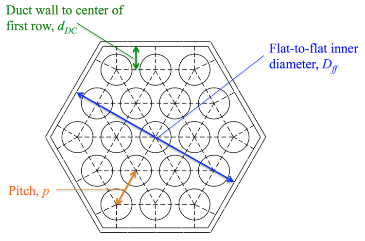
Figure 3.19.6 Assembly Layout Diagram

3.19.2.2.1.1. Basic Dimensions Calculation

Depending on the choice of preprocessor inputs IPDOPT and ISC, the SAS4A/SASSYS‑1 input for the channel geometry will be calculated differently. In any case, the basic geometric inputs listed in Table 3.19.5 are then used to calculate additional geometric information, such as those variables listed in Table 3.19.6. Some of these variables are needed for direct SAS4A/SASSYS‑1 input, such as ACCZ, while others are used to calculate other variables in the following sections, such as the flow splits or subassembly-to-subassembly heat transfer coefficients.

Table 3.19.5 Preprocessor Input Geometric Variables

Symbol	Input	Description
\(D_{\text{ff}}\)	FFID	Flat-to-flat inner diameter
\(d_{\text{DC}}\)	DEDGE	Distance from duct wall to center of 1st row of pins
\(D_{\text{pin}}\)	DPIN	Diameter of pin
\(D_{\text{WW}}\)	DWW	Diameter of wrapper wire
\(p\)	PITCH	Pin centerline to centerline distance
\(l_{\text{WW}}\)	HWW	Wrapper wire lead length
\(t_{C}\)	DRE	Thickness of clad
\(t_{\text{DW}}\)	TDW	Thickness of duct wall
\(t_{\text{GAP}}\)	TGAP	Thickness of gap between subassemblies

Table 3.19.6 Calculated Geometric Variables

Symbol	Variable	Description
\(A_{\text{pin}}\)		Area of pin
\(A_{\text{WW}}\)		Area of wrapper wire
\(P_{\text{WW}}\)		Perimeter of wrapper wire
\(A_{\text{hex}}\)		Area of subassembly hex
\(P_{\text{hex}}\)		Perimeter of subassembly hex
\(A_{\text{CC}}\)	ACCZ	Cross-sectional flow area per pin
\(D_{h}\)	DHZ	Hydraulic diameter

3.19.2.2.1.2. Flow Splits Calculation

The flow split calculation starts with establishing the exponential variable \(\alpha\), which is calculated using the preprocessor input BFR. BFR is also used in SAS4A/SASSYS‑1 for the calculation of the turbulent friction factor.

(A3.2‑1)

\[\alpha = \frac{1 - \text{BFR}}{2 + \text{BFR}}\]

From there, the flow split per region \(f_{\text{XX}}\) can be calculated using the following equation, where XX is the region abbreviation seen in Table 3.19.1.

(A3.2‑2)

\[f_{\text{XX}} = A_{\text{CC}_{\text{XX}}}D_{\text{h}_{\text{XX}}}^{\alpha}\]

Table 3.19.7 Region Abbreviations

Abbreviation - XX	Region
INR	Inner Row of Subchannels
INB	Inner Subchannels (except inner row if IPDOPT = 3)
RN	Corner Subchannels
ED	Edge Subchannels

The total flow area can be found from Table 3.19.8, where each value in the right hand column is added to the total flow area.

Table 3.19.8 Total Flow Area Contributions

Region		Amount Added to Total Flow Area
INR		\(3f_{\text{INR}}\)
INB	If \(n_{\text{rows}} = 1\), If \(n_{\text{rows}} \neq 1\),	\(f_{\text{INB}}\) \((3 - 6n_{\text{rows}} + 3n_{\text{rows}}^{2} - 3^{*})f_{\text{INB}}\)
RN		\(f_{\text{RN}}\)
ED	If \(n_{C_{\text{RN}}} > 0\), If \(n_{C_{\text{RN}}} = 0\),	\(\left( 3\left( n_{\text{rows}} - 1 \right) \right)f_{\text{ED}}\) \(\left( 1 + 3\left( n_{\text{rows}} - 1 \right) \right)f_{\text{ED}}\)

* Subtract 3 only if the number of inner subchannels > 0

Then the normalized initial coolant flow split \(w_{\text{N}_{\text{XX}}}\) is the value of the flow split for region XX divided by the total flow area, determined by Table 3.19.8, times the total core flow \(w_{\text{core}}\) , which is defined by the preprocessor input WTOTL.

(A3.2‑3)

\[w_{\text{N}_{\text{XX}}} = \left( \frac{f_{\text{XX}}}{\text{Total}} \right)w_{\text{core}}\]

If bypass subchannels (thimble flow corners) are present, the same process holds, where XX is the region from Table 3.19.9.

(A3.2‑4)

\[f_{\text{XX}} = A_{\text{CC}_{\text{XX}}}D_{\text{h}_{\text{XX}}}^{\alpha}\]

Table 3.19.9 Bypass Region Abbreviations

Abbreviation	Region
BYE	Bypass Edge Subchannels
BYC	Bypass Corner Subchannels

The total bypass flow area can be found from Table 3.19.10

Table 3.19.10 Total Bypass Flow Area Contributions

Region		Amount Added to Total Bypass Flow Area
BY	If ISC = 3 If ISC = 5 If ISC = 6	\({6f}_{\text{BYE}}\) \({6\left( n_{\text{rows}} - 1 \right)f}_{\text{BYE}}\) \(f_{\text{BYE}}\)
NR	If ISC = 3 If ISC = 5 If ISC = 6	\(0\) \(6f_{\text{NR}}\) \(0\)

The bypass normalized initial coolant flow split is then just the regional flow split divided by the total bypass flow area, multiplied by the total bypass flow \(w_{\text{bypass}}\), which is defined by the preprocessor input WBYFL.

(A3.2‑5)

\[w_{\text{N}_{\text{XX}}} = \left( \frac{f_{\text{XX}}}{\text{Total}_{\text{bypass}}} \right)w_{\text{bypass}}\]

3.19.2.2.2. Subchannel-to-Subchannel Heat Flow Coefficients

For the multiple pin options (ISC = 2, 3, 4, or 5), the subchannel-to-subchannel heat flow coefficients must be determined (Eq. 3.14-7 in Section 3.14.2). The SAS4A/SASSYS‑1 input UACHM1, which is used in the coolant subchannel-to-subchannel heat flow per pin unit height calculation, can be split into coolant and clad contributions, as explained in Section 3.14.2,

(A3.2‑6)

\[\text{UACHM}1_{\text{total}} = \text{UACHM}1_{\text{XXXX}} + \text{UACHM}1_{\text{Clad}}\]

where \(\text{UACHM}1_{\text{XXXX}}\) is the coolant contribution from the XXXX region, and \(\text{UACHM}1_{\text{Clad}}\) is the contribution from the cladding. The regions are described in Table 3.19.11.

Table 3.19.11 Region Abbreviations

Abbreviation - XXXX	Region
ININ	Inner row to inner row
IAIA	Inner average row to inner average row
IAE	Inner average row to edge
INIA	Inner row to inner average row
EDED	Edge to edge
EDCN	Edge to corner

The clad contribution is independent of the region, and is defined below, where \(k_{\text{ww}}\) is the thermal conductivity of the wrapper wire (preprocessor input XKSS), \(M\) is a multiplier (preprocessor input FU1E), and \(k_{\text{gap}}\) is the thermal conductivity of the coolant in the gap (preprocessor input XKGAP).

(A3.2‑7)

\[\text{UACHM}1_{\text{Clad}} = \frac{12k_{\text{ww}}t_{\text{c}}M}{\pi k_{\text{gap}}D_{\text{pin}}}\]

The coolant contribution to UACHM1 depends on the region, and uses the following equations for each of the regions defined in Table 3.19.11,

(A3.2‑8)

\[\text{UACHM}1_{\text{ININ}} = \left( \frac{0.774D_{\text{ww}}\left( D_{\text{pin}} + D_{\text{ww}} \right)}{\left( \frac{D_{\text{pin}} + D_{\text{ww}}}{\sqrt{3}} \right)D_{\text{pin}}} \right)\left( \frac{D_{\text{ww}}}{D_{\text{pin}}} \right)^{- 0.2627}\]

(A3.2‑9)

\[\text{UACHM}1_{\text{IAIA}} = \left( \frac{0.774\left( p - D_{\text{pin}} \right)p}{\frac{p}{\sqrt{3}}D_{\text{pin}}} \right)\left( \frac{p - D_{\text{pin}}}{D_{\text{pin}}} \right)^{- 0.2627}\]

(A3.2‑10)

\[\text{UACHM}1_{\text{IAE}} = \text{UACHM}1_{\text{IAIA}}\]

(A3.2‑11)

\[\text{UACHM}1_{\text{INIA}} = \left( \frac{0.774D_{\text{ww}}\left( D_{\text{pin}} + D_{\text{ww}} \right)}{\left( \frac{\frac{p}{\sqrt{3}} + \frac{D_{\text{pin}} + D_{\text{ww}}}{\sqrt{3}}}{2} \right)D_{\text{pin}}} \right)\left( \frac{D_{\text{ww}}}{D_{\text{pin}}} \right)^{- 0.2627}\]

(A3.2‑12)

\[\text{UACHM}1_{\text{EDED}} = \frac{1}{2}\left( \frac{0.774\left( 2\left( p - D_{\text{pin}} \right) \right)p}{pD_{\text{pin}}} \right)\left( \frac{2\left( p - D_{\text{pin}} \right)}{D_{\text{pin}}} \right)^{- 0.2627}\]

(A3.2‑13)

\[\text{UACHM}1_{\text{EDCN}} = \frac{1}{2}\left( \frac{0.774\left( 2\left( p - D_{\text{pin}} \right) \right)p}{{\left( \frac{p}{2} + \frac{d_{\text{DC}}}{\sqrt{3}} \right)D}_{\text{pin}}} \right)\left( \frac{2\left( p - D_{\text{pin}} \right)}{D_{\text{pin}}} \right)^{- 0.2627}\]

The SAS4A/SASSYS‑1 input UACHM2, which is used in the coolant subchannel-to-subchannel heat flow per pin unit height calculation, can be found by the following (if IPODPT = 3) for inner row to inner row heat flow,

(A3.2‑14)

\[\text{UACHM}2_{\text{ININ}} = \frac{\text{CXTC}*D_{\text{ww}}}{2A_{\text{CC}_{\text{INR}}}}\]

and for the inner row to the inner average, (\(\text{UACHM}2_{\text{ININ}}\) and \(\text{UACHM}2_{\text{INIA}}\) are zero for IPODPT \(\neq 3\))

(A3.2‑15)

\[\text{UACHM}2_{\text{INIA}} = \frac{\text{CXTC}*D_{\text{ww}}}{A_{\text{CC}_{\text{INR}}} + A_{\text{CC}_{\text{INB}}}}\]

For all IPODPT options, the inner average to inner average value follows,

(A3.2‑16)

\[\text{UACHM}2_{\text{IAIA}} = \frac{\text{CX}*(p - D_{\text{pin}})}{2A_{\text{CC}_{\text{INB}}}}\]

For the inner average to the edge,

(A3.2‑17)

\[\text{UACHM}2_{\text{IAE}} = \frac{\text{CX}*(p - D_{\text{pin}})}{A_{\text{CC}_{\text{INB}}} + A_{\text{CC}_{\text{ED}}}}\]

The value for UACHM2 for both edge to edge, and edge to corner heat flow is zero. The placeholder variables are defined below,

(A3.2‑18)

\[\text{CXTC} = \text{CMMTC}\left( \text{TAN}\text{SQR}*\frac{\text{AR}1}{A1\text{PTC}} \right)^{\frac{1}{2}}\]

(A3.2‑19)

\[\text{CX} = \text{CMT}\left( \text{TANSQR}*\frac{\text{AR}1}{A1\text{PTC}} \right)^{\frac{1}{2}}\]

(A3.2‑20)

\[\begin{split}\begin{aligned} \text{CMMTC} = 0.1 \frac{D_{\text{ww}}}{D_{\text{pin}}}^{- \frac{1}{2}} && \text{If } n_{\text{SA}} < 7 \\ \text{CMMTC} = 0.14\frac{D_{\text{ww}}}{D_{\text{pin}}}^{- \frac{1}{2}} && \text{If } n_{\text{SA}} \geq 7 \\ \end{aligned}\end{split}\]

(A3.2‑21)

\[\begin{split}\begin{aligned} \text{CMT} = 0.1 \left( \frac{p - D_{\text{pin}}}{D_{\text{pin}}} \right)^{- \frac{1}{2}} && \text{If } n_{\text{SA}} < 7 \\ \text{CMT} = 0.14\left( \frac{p - D_{\text{pin}}}{D_{\text{pin}}} \right)^{- \frac{1}{2}} && \text{If } n_{\text{SA}} \geq 7 \\ \end{aligned}\end{split}\]

(A3.2‑22)

\[\text{TANSQR} = \frac{1}{\left( \frac{h_{\text{ww}}}{\sqrt{h_{\text{ww}}^{2} + \left( \pi\left( D_{\text{pin}} + D_{\text{ww}} \right) \right)^{2}}} \right)^{2}}\]

(A3.2‑23)

\[\text{AR}1 = \frac{\pi\left( D_{\text{pin}} + D_{\text{ww}} \right)D_{\text{ww}}}{6}\]

(A3.2‑24)

\[\text{A}1\text{PTC} = \frac{1}{4}p^{2}\sqrt{3} - \frac{\pi D_{\text{pin}}^{2}}{8}\]

For swirl flow, the SAS4A/SASSYS‑1 input XKSWRL, which is used to calculate swirl flow between subchannels, can be found using the following for the edge to edge calculation,

(A3.2‑25)

\[\text{XKSWR}L_{\text{EDED}} = \frac{C1L(p - D_{\text{pin}})}{A_{\text{CC}_{\text{ED}}}\beta}\]

where,

(A3.2‑26)

\[\begin{split}\begin{aligned} \beta = \frac{1}{2} && \text{If } \text{ISC} > 3 \\ \beta = \frac{1}{6} + \frac{1}{2}\left( n_{\text{rows}} - 1 \right) && \text{If } \text{ISC} \leq 3 \\ \end{aligned}\end{split}\]

For XKSWRL from the edge to corner,

(A3.2‑27)

\[\text{XKSWRL}_{\text{EDCN}} = \text{XKSWRL}_{\text{EDED}}\]

Lastly, the value for XKSWRL from the corner to edge depends on the selection for ISC,

(A3.2‑28)

\[\begin{split}\begin{aligned} \text{XKSQRL}_{\text{CNED}} = \frac{6(\text{C}1\text{L})(p - D_{\text{pin}})}{A_{\text{CC}_{\text{CN}}}} && \text{If } \text{ISC} > 3 \\ \beta = \text{XKSWRL}_{\text{CNED}} = \text{XKSWRL}_{\text{EDED}} && \text{If } \text{ISC} \leq 3 \\ \end{aligned}\end{split}\]

Where the placeholder variables are defined below,

(A3.2‑29)

\[\text{C}1\text{L} = \text{CST}\left( \text{TANSQR}\left( \frac{\left( \frac{3}{2} \right)\pi\left( D_{\text{pin}} + D_{\text{ww}} \right)\left( \frac{D_{\text{ww}}}{6} \right)\ }{pd_{\text{DC}} - \frac{\pi D_{\text{pin}}^{2}}{8}} \right) \right)^{\frac{1}{2}}\]

(A3.2‑30)

\[\begin{split}\begin{aligned} \text{CST} = 0.1 \left( \frac{h_{\text{ww}}}{D_{\text{pin}}} \right)^{0.3} && \text{If } n_{\text{SA}} < 7 \\ \text{CST} = 0.75\left( \frac{h_{\text{ww}}}{D_{\text{pin}}} \right)^{0.3} && \text{If } n_{\text{SA}} \geq 7 \\ \end{aligned}\end{split}\]

The calculation of the SAS4A/SASSYS‑1 input ALATRL, which is the coolant lateral flow area per pin, depends greatly on the pin options chosen by ISC and IPDOPT, with too many possible combinations to review in this document.

3.19.2.2.3. Subassembly-to-Subassembly Heat Transfer

Before the subassembly-to-subassembly heat transfer calculations can be conducted, a series of more detailed geometric variables must be found that includes many SAS4A/SASSYS‑1 inputs. These variables, shown in Table 3.19.12, are calculated using the basic geometric information found in Section 3.19.2.2.1.

Table 3.19.12 Detailed Geometric Variables

Block	Variable	Description
GEOMIN	RER0	Nominal cladding outer radius
	RBR0	Nominal cladding inner radius
	DRF0	Thickness of the outer reflector node
	DRFI	Thickness of the inner reflector node
	SER	Reflector perimeter per pin wetted by coolant
	RBRPL	Cladding inner radius in gas plenum
	RERPL	Cladding outer radius in gas plenum
	AREAPC	Coolant plus pin area per pin
	SRFSTZ	Structure perimeter
	DSTIZ	Thickness of inner structure node
	DSTOZ	Thickness of outer structure node
POWINC	PRSHAP	Ratio of power per subassembly
PMATCH	XKSTIZ	Inner structure thermal conductivity
	XKSTOZ	Outer structure thermal conductivity
	RHOCSI	Density*heat capacity for the inner structure
	RHOCSO	Density*heat capacity for the outer structure
	RHOCR	Density*heat capacity for the reflector
	XKRF	Thermal conductivity of reflector/cladding (in gas plenum)
COOLIN	W0	Steady-state coolant flow rate per fuel-pin

3.19.2.2.3.1. Single-Pin Options

For the single pin treatment with no bypass channel (ISC = 0 or 1), the preprocessor will only calculate subassembly-to-subassembly heat transfer if the channel represents one subassembly. If the channel represents more than one subassembly, this input must be calculated manually. The first step for calculating subassembly-to-subassembly heat transfer is to determine which subassemblies are in contact. Using the core symmetry option ISYM and the number of rows NROW, the preprocessor finds the six adjacent assemblies. The preprocessor resolves whether a subassembly is at an adiabatic boundary.

Once the adjacent subassemblies are known, the SAS4A/SASSYS‑1 input related to subassembly heat transfer, shown in Table 3.19.13, is calculated for each flat of the subassembly. This information is then printed to the preprocessor output in the correct format for insertion into a SAS4A/SASSYS‑1 input deck.

Table 3.19.13 Subassembly Heat Transfer SAS Inputs

Block	Variable	Description
INPCHN	NCHCH	Number of other channels in contact
INPCHN	ICHCH	Channel number that is in contact
INPCHN	IOPCHC	Subassembly to subassembly heat transfer option
PMATCH	HACHCH	Heat-transfer coefficient x area per unit height

For the single pin treatment with bypass channel (ISC = 6), the additional geometric parameters relating to the bypass channel are found, and then the adjacent subassemblies are determined. From there, the process follows a similar path as the single pin options with no bypass channel, where the variables in Table 3.19.13 are found (but taking into account the bypass) and the output is printed.

3.19.2.2.3.2. Multiple-Pin Options

The calculation process is more complicated for the multi-pin options (ISC = 2, 3, 4, or 5). For each row of pins, the detailed geometric variables in Table 3.19.11 are calculated. The power gradient is found first using the preprocessor input IDRGRD. This information, along with the preprocessor input PRSHP0, is necessary to calculate the SAS4A/SASSYS‑1 input POWINC:PRSHAP. The formulas used to calculate the variables in Table 3.19.11 differ depending on the choice of IPDOPT and ISC (whether grouped by sector and row or individual subchannels). Where the channel is located, whether it is an inner, edge, or corner channel, also affects the calculation. The location is determined using the number of rows NROW and the choices for IPDOPT and ISC. This is also used to calculate the SAS4A/SASSYS‑1 input JCHMPN, which denotes what channels are in contact.

The heat flow parameters found in Section 3.19.2.2.2 are then adjusted (normalized) for the different pin nodes. The calculation of the subassembly heat transfer variables in Table 3.19.12 is also more intricate than the single pin models, and depends on whether individual subchannels are being used (ISC = 4, 5) or subchannels grouped by row and sector (ISC = 2, 3).

3.19.2.3. User Guide

3.19.2.3.1. Overview

The current preprocessor is useful for a limited subset of the cases that SAS4A/SASSYS‑1 can handle, as shown in Table 3.19.14. The current preprocessor was written only for hexagonal subassemblies with solid duct walls and wire wrapped pins. A modified preprocessor would be needed to handle square arrays, pins with grid spacers instead of wire wraps, or ductless subassemblies. Also, the preprocessor does not handle subassembly-to-subassembly heat transfer involving a channel that represents more than one subassembly.

Table 3.19.14 Scenarios Covered by Preprocessor

Covered	Not Covered
Hexagonal Subassemblies Solid Duct Walls Wire Wrapped Pins	Square Subassemblies Ductless Subassemblies Pins with Grid Spacers

The current preprocessor provides input only for the pin section of a subassembly. Input for the reflector zones above and below the pin section must be input into SAS4A/SASSYS‑1 manually, as shown in Figure 3.19.7, but such information only needs to be input once for each subassembly type, as explained in Section 3.15.3.1.

The preprocessor numbers the channels in a consistent manner, and determines subchannel connectivity. In the pin zone the preprocessor calculates three types of parameters. As described in Section 3.19.2.2, it first calculates geometrical parameters, such as coolant flow areas and hydraulic diameters. Second, it uses correlations to calculate the parameters used for subchannel-to-subchannel heat flow. Third, it calculates the parameters used in subassembly-to-subassembly heat transfer.

The preprocessor can also print additional user-specified information directly to the created SAS4A/SASSYS‑1 input in order to help reduce the time needed to create the SAS4A/SASSYS‑1 input. This allows a block of text to be input once into the preprocessor, which then duplicates that text for all channels of that type. This is done through the ICARD option, and is explained in more detail in Section 3.19.2.2.3 and Section 3.19.2.3.5.

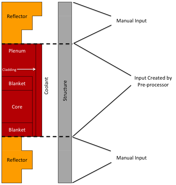
Figure 3.19.7 Preprocessor Coverage

The preprocessor could be of some use even if the three dimensional core thermal hydraulics model is not being used. For a single average channel treatment, the preprocessor can calculate the geometrical parameters such as coolant flow areas and hydraulic diameters for each subassembly. Also, if a separate channel represents each subassembly, then input for subassembly-to-subassembly heat transfer can be calculated by the preprocessor.

3.19.2.3.2. Input/Output Format

The layout of the input file can be broken into three main sections, as shown in Figure 3.19.8. The general input is first, then the subassembly type(s) information, which can also include the optional visualization input, followed by the individual subassembly information. This last section can also include the ICARD information if the preprocessor options ICD or ICDBFR are being used, which allow additional text to be added to the preprocessor output.

Table 3.19.15 provides more detail about the input structure, beginning with the general input. Each subassembly type must have its ITYPE value in consecutive order. Then, ITYPE = 0 is used to signal the end of the subassembly type input. Also, the optional visualization input is entered independently for each subassembly type. A similar structure is used for the subassembly input, where the value for ISUBAS must be in consecutive order, and ISUBAS = 0 signals the end of the subassembly input. The optional ICARD data is entered independently for each subassembly. The format of the input is described in Table 3.19.16.

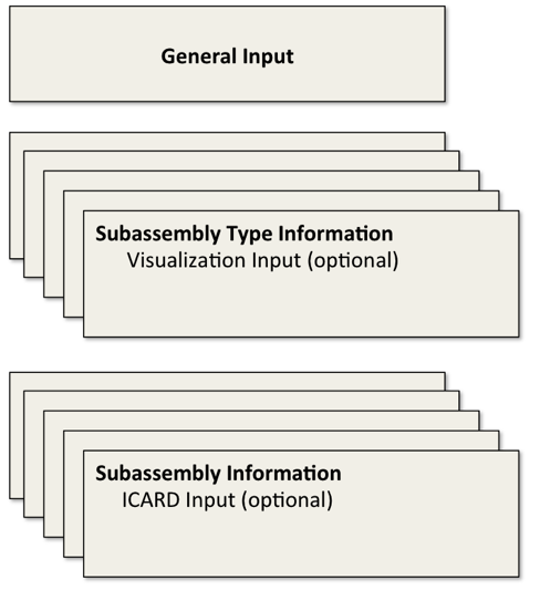
Figure 3.19.8 Preprocessor Input Layout

Table 3.19.15 Preprocessor Input Structure

General Input
1st Subassembly Type Input (ITYPE = 1)
	Visualization Input (optional)
2nd Subassembly Type Input (ITYPE = 2)
	Visualization Input (optional)
…
Last Subassembly Type Input
	Visualization Input (optional)
ITYPE 0
1st Subassembly Input (ISUBAS = 1)
	ICARD Input (optional)
2nd Subassembly Input (ISUBAS = 2)
	ICARD Input (optional)
…
Last Subassembly Input
	ICARD Input (optional)
ISUBAS 0

Table 3.19.16 Preprocessor Input Formatting

Section/Variable	Fortran Format
General Input
ITITLE	(A80)
NROW, ISYM, IFSTCH, IHEXPL, IHEXP2, IDBUG, IFSTSA	7(7X,I5)
Subassembly Type Input
ITYPTL	(A80)
ITYPE, ISC(ITYPE), NPINSB(ITYPE), IPDOPT(ITYPE), KZPIN(ITYPE), IBYOPT(ITYPE), ISWDIR(ITYPE)	7(7X,I5)
DPIN(ITYPE), DWW(ITYPE), PITCH(ITYPE), DEDGE(ITYPE)	4(10X,F10.5)
FFID(ITYPE), HWW(ITYPE), TBY(ITYPE), TDWBY(ITYPE)	4(10X,F10.5)
AFR(ITYPE), BFR(ITYPE), AFLAM(ITYPE), RELAM(ITYPE)	4(10X,F10.5)
DRE(ITYPE), FU1E(ITYPE), HCBY(ITYPE)	3(10X,F10.5)
TDW(ITYPE), TGAP(ITYPE), RHOCSS(ITYPE), RHOCNA(ITYPE)	4(10X,E10.3)
XKSS(ITYPE), XKGAP(ITYPE), FRSTIN(ITYPE), FRSTED(ITYPE)	4(10X,E10.3)
Visualization Input (optional)
LDETL(ITYPE), MZ(ITYPE), NT(ITYPE), IEQMAS(ITYPE)	6(7X,I5)
(ZMZ(IZ,ITYPE),IZ=1,MZ)	(6E12.5)
RINFP, ROUTFP	(2E12.5)
Subassembly Input
ISUBAS, ITYPEV(ISUBAS), KMAX, IDRGRD(ISUBAS), NSUB(ISUBAS), ICD(ISUBAS)	6(7X,I5)
SATITL	(A80)
ICDBFR, IHTLAT(ISUBAS)	2(7X,I5)
WTOTL(ISUBAS), PRSHP0(ISUBAS), PGRAD(ISUBAS), ADOPPN(ISUBAS)	4(10X,F10.6)
BDOPPN(ISUBAS), WBYFL(ISUBAS), HALATP(ISUBAS)	3(10X,F10.6)
(IHXPSS(K), IHXPSE(K),K=1,KMAX)	(20X,12I5)
NPRINT, (ICHPRT(I,ISUBAS),I=1,NPRINT)	(20x,12I5)

3.19.2.3.3. Input Description

As stated in Section 3.19.2.3.2 and shown in Table 3.19.17, the input for the preprocessor can be split into three major sections with the visualization input under the subassembly type section. The following tables outline the input for each section. The input needed for the visualization tool, described in Section 3.19.3, is also provided.

Table 3.19.17 Preprocessor Input Sections

Section	Description
General Input	General Input
Subassembly Type Input	Specifies pin treatment and geometric options for each subassembly type
Visualization Input (optional)	Specifies details for creation of visualization mesh, described in Section 3.19.3
Subassembly Input	Subassembly specific data

General Input
Symbol	Description
ITITLE	One line of title information. (80 character limit)
NROW	Number of rows of subassemblies in the model.
ISYM	Symmetry information = 1, Full core = 2, Half core = 3, Third core = 4, Quarter core = 6, Sixth core = 12, 1/12 core
IFSTCH	First channel number to use.
IHEXPL	Plot information = 0, Skip plot of subassembly hexes numbered with hex positions for the symmetry and number of rows being used = 1, Plot to file HEX_NUM.ps and continue = 2, Plot to file HEX_NUM.ps and quit
IHEXP2	Plot information = 0, Skip plot of subassembly hexes numbered with subassembly numbers > 0, Plot subassembly hexes numbered with subassembly numbers to file SUB_NUM.ps. = 2, Generate visualization geometry file for use with VisIt, additional input must be provided as described in Section 3.19.3
IDBUG	Debugging output > 0, Debugging output
IFSTSA	First subassembly number to use.

Subassembly Type Input
Symbol	Description
ITYPTL	One line of type title information. (80 character limt)
ITYPE	Subassembly type. If ITYPE=0, this is the end of the type input.
ISC (ITYPE)	Pin treatment option = 0, JJMLTP = 0, No multi-pin treatment = 1, JJMLTP = 1, 1 pin treatment = 2, Multi-pin, subchannels grouped by row and sector = 3, Multi-pin, same as 2, but bypass flow channel on outside = 4, Multi-pin, individual subchannels = 5, Multi-pin, individual subchannels, bypass flow channel on the outside = 6, JJMLTP = 1, 1 pin treatment, bypass flow channel
NPINSB (ITYPE)	Number of pins per subassembly.
IPDOPT (ITYPE)	Geometry Calculation Options = 0, Use input PITCH everywhere, calculate DEDGE based on what is left over, use input FFID = 1, Use FFID, calculate uniform PITCH, DEDGE = 2, Use input PITCH, calculate DEDGE with same slop, calculate FFID = 3, Hit channel option: use FFID, use: P = DPIN + DWW for 1 inner row of subchannels, use PITCH for other inner subchannels, calculate DEDGE based on what is left over = 4, Use PITCH and DEDGE, calculate FFID
KZPIN (ITYPE)	Zone KZ
IBYOPT (ITYPE)	Bypass information = 0, Bypass flow the whole length of the subassembly = 1, Bypass flow only in the pin section Note: IBYOPT is only relevant if ISC = 3, 5, or 6. IBYOPT = 1 is not currently implemented
ISWDIR (ITYPE)	Swirl information = 1, Swirl flow is counter-clockwise, when viewed from above = 2, Swirl flow is clockwise
DPIN (ITYPE)	Pin Diameter.
DWW (ITYPE)	Wrapper wire diameter.
PITCH (ITYPE)	Pin Centerline to Centerline Distance.
DEDGE (ITYPE)	Distance from duct wall to center of first row of pins.
FFID (ITYPE)	Flat-to-flat ID.
HWW (ITYPE)	Wire wrap lead length.
TBY (ITYPE)	Thickness of bypass flow gap.
TDWBY (ITYPE)	Thickness of the outer duct wall beyond the bypass gap.
AFR (ITYPE)	Turbulent Friction Factor = AFR*Re**BFR
BFR (ITYPE)	Turbulent Friction Factor = AFR*Re**BFR
AFLAM (ITYPE)	Laminar Friction Factor = AFLAM/Re
RELAM (ITYPE)	Reynolds number for transition from turbulent to laminar. If RELAM = 0, then it is calculated so that turbulent friction factor equals laminar friction factor at RELAM.
DRE (ITYPE)	Clad thickness.
FU1E (ITYPE)	Geometry multiplier for subchannel-to-subchannel heat transfer by conduction through cladding. Typical value near 2.0.
HCBY (ITYPE)	Coolant heat transfer coefficient from outer surface of duct wall to thimble flow coolant. For laminar flow, HCBY = 7.6*k/Dh to 8.23*k/Dh.
TDW	Thickness of duct wall.
TGAP	Thickness of gap between subassemblies.
RHOCSS	Density × heat capacity of the wrapper wire and duct wall.
RHOCNA	Density × heat capacity of the coolant in the gap.
XKSS	Thermal conductivity of the wrapper wire and duct wall.
XKGAP	Thermal conductivity of the coolant in the gap.
FRSTIN	Fraction of structure thickness in the inner node, inner subchannel.
FRSTED	Fraction of structure thickness in the inner node, edge subchannel.
Visualization Input (if IHEXP2 = 2) 4
Symbol	Description
LDETL	Level of detail in the visualization mesh geometry file. = 0, Do not generate geometry for this assembly type. = -1, Only simplified coolant subchannels are defined. = -2, Simplified coolant subchannels and duct wall structure. = 1, Detailed coolant subchannels are defined. = 2, Detailed coolant subchannels and duct wall structure. = 3, Detailed subchannels, duct wall, and simple fuel pin. = 4, Detailed subchannels, duct wall, and detailed fule pin.
MZ	Number of axial segments in zone KZPIN (e.g., the MZ mesh).
NT	Number of radial temperature nodes within the fuel (only relevant for LDETL = 4).
IEQMAS	Radial fuel mesh size assumptions (relevant for LDETL=4). = 0, Equal radial distance. > 0, Equal cylindrical area.
ZMZ	Axial segment boundaries for zone KZPIN, where the lowest boundary is assumed to be zero. Note that these and the above values are only used to generate the geometry file, and are not used to define NZNODE, AXHI, or ZONEL.
RINFP	Fuel inner radius.
ROUTFP	Fuel outer radius (default = clad inner radius)

Subassembly Input
Symbol	Description
ISUBAS	Subassembly number. Max = NSBMAX = 1000. If ISUBAS = 0, then this is the end of the subassembly input.
ITYPEV (ISUBAS)	ITYPE = subassembly type.
KMAX	Highest pin axial node, as shown in Figure 3.15.4
IDRGRD (ISUBAS)	Direction of power gradient. = 1, N(high) - S(low) = 2, NNE - SSW = 3, NE - SW = 4, E - W = 5, SE - NW = 6, SSE - NNW
NSUB (ISUBAS)	Number of real subassemblies represented by this ISUBAS
ICD	If > 0, Read in cards, ICARD, to be put at the end of the first channel in ISUBAS
SATITL (ISUBAS)	Subassembly title information.
ICDBFR	If > 0, Read in cards to be put before the first channel in ISUBAS.
IHTLAT	If > 0, Use HALATP(ISUBAS) for lateral heat transfer across pins. Currently, only implemented for the detailed subchannel treatment (ISC = 4 or 5). Not implemented for the one pin per subassembly case.
WTOTL (ISUBAS)	Total subassembly coolant flow, excluding thimble flow.
PRSHP0 (ISUBAS)	Average PRSHAP for the subassembly. PRSHAP = Ratio of power per subassembly averaged over this channel to the power per subassembly averaged over all channels.
PGRAD (ISUBAS)	Power gradient. \(\text{PRSHAP}\ = \ \frac{\text{PRSHP}0\left( 1 + \text{PGRAD} \right)\text{XPIN}}{\text{NPINSB}}\) at SA 5 Edge \(\text{PRSHAP}\ = \ \frac{\text{PRSHP}0\ \times \ \text{XNPIN}}{\text{NPINSB}}\) at SA Center \(\text{PRSHAP}\ = \ \frac{\text{PRSHP}0\left( 1 - \text{PGRAD} \right)\text{XPIN}}{\text{NPINSB}}\) at SA Other Edge
ADOPPN	ADOP per pin. ADOP = Doppler coefficient for this channel when part of the core represented by this channel is not voided.
BDOPPN	BDOP per pin. BDOP = Doppler coefficient for this channel when part of the core represented by this channel is fully voided.
WBYFL	Total thimble flow. Used only if ISC = 3, 5, or 6.
HALATP	Heat transfer coefficient × area/height for lateral heat transfer across pins.
IHXPSS	Subassembly ISUBAS represents subassemblies with hex position numbers from IHXPSS(K) to IHXPSE(K)
IHXPSE	See above
NPRINT	Number of channels in this subassembly which will be printed out in normal prints (set IPRSKP = 0, in all other channels IPRSKP will be set to 1).
ICHPRT	Relative channel number (1 for the first channel in the subassembly).
ICARD	Information to be read and directly printed to fort.1 output. See ICD and ICDBFR.

3.19.2.3.4. Input Example

An example input is provided in Figure 3.19.9, where “#” is used as a placeholder for user specified values. This example has two subassembly types, and two subassemblies. The visualization tool is also used for both subassembly types. The two subassemblies use the ICARD option, with the first subassembly (ISUBAS = 1) using ICDBFR, and the second subassembly (ISUBAS = 2) using ICD.

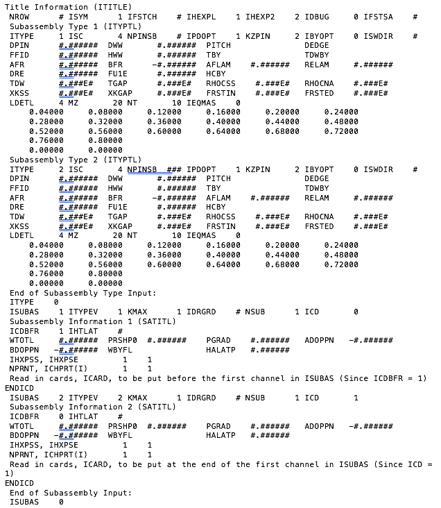
Figure 3.19.9 Preprocessor Example Input

3.19.2.3.5. Output Description

Lastly, several output files are created by the preprocessor, as seen in Table 3.19.18. The first output file is the direct output from the preprocessor, which documents notifications printed during its execution. The second file, fort.1 is the SAS4A/SASSYS‑1 input created by the preprocessor. If the ICARD option is being used (ICD or ICDBFR > 0), then ICARD information will be printed directly to fort.1. The location of the ICARD information will be before the first channel in ISUBAS if ICDBFR is being used, or at the end of the first channel in ISUBAS if ICD is used.

The preprocessor can optionally produce postscript plots to HEX_NUM.ps and SUB_NUM.ps. HEX_NUM.ps plots the subassembly hexes numbered with the position numbers used internally by the preprocessor. SUB_NUM.ps plots the subassembly hexes numbered with the subassembly numbers assigned by the user. The two plots could be identical if the user picks the same numbering scheme that the preprocessor uses internally. Lastly, the optional visualization geometry file, SAS.sasgeom, can be created. More details on this file can be found in Section 3.19.3.

Table 3.19.18 Output File Description

Output	Description
*.out	Log
fort.1	SAS4A/SASSYS‑1 input
HEX_NUM.ps	Plot of the subassembly hexes numbered with the position numbers used internally by the preprocessor (postscript)
SUB_NUM.ps	Plot of the subassembly hexes numbered with the subassembly numbers assigned by the user (postscript)
SAS.sasgeom	Visualization mesh file (optional)

3.19.3. APPENDIX 3.3: Visualization

3.19.3.1. Introduction

An advanced visualization capability has been developed for the SAS4A/SASSYS‑1 code [1] that allows for the generation, display, and animation of large datasets that are calculated during a transient simulation. The key features of the new capability include its support for multiple-pin, subchannel modeling, integration with the subchannel input preprocessor, geometry visualization, fully-detailed temperature field support with unlimited dataset sizes, and interactive visualization and animation generation on a desktop PC using the visualization tool VisIt [2].

The motivation for developing an advanced visualization capability results from the ever-increasing fidelity with which fast reactor transient simulations are being carried out and the enormous amounts of data generated during those simulations. For example, the EBR-II SHRT-17 test has recently been modeled [3] with subchannel-level detail and a coarse axial mesh for the experimental assembly XX09 and its six nearest neighbors. For a simulation that lasts 250 seconds with data saved every one-tenth of a second, the full temperature field in the active core region for these seven assemblies is estimated to be approximately 15 GB. 6 While it is trivial to identify maxima and minima within this large dataset, identifying other features is much more difficult. Items of interest might include the identification of power, flow, or temperature fluctuations caused by instabilities in the numerical solution, regions of temperature near (but not at) the peak, flow reversals at the subchannel level, unusual results caused by input error, time-derivatives of solution variables, and so on.

The following sections describe changes made to the subchannel input preprocessor to support creation of visualization mesh geometry and preliminary changes made to the SAS4A/SASSYS‑1 code to support large dataset generation. Finally, examples of using the visualization tool VisIt to render three-dimensional images from the SHRT-17 simulation are provided.

3.19.3.2. Mesh Generation

Channel modeling in the SAS4A/SASSYS‑1 code is fundamentally based on a single-pin representation that includes associated coolant and structure. Geometric input to the SAS4A/SASSYS‑1 code is represented by generalized parameters such as flow area, hydraulic diameter, heat-transfer area, etc, and details of the problem-specific geometry are not fully known. In order to project computed transient data into three-dimensional space, a visualization mesh representing the actual geometry of the problem needs to be defined.

Detailed core models using the multiple-pin subchannel capability in the SAS4A/SASSYS‑1 safety analysis code are usually created using the subchannel input preprocessor, detailed in Section 3.19.2. The input preprocessor takes subassembly design information and creates detailed SAS4A/SASSYS‑1 input descriptions of the multiple-pin subchannels in terms of geometric, thermal, and hydraulic parameters. Because the input preprocessor contains subassembly design information that is not available to the SAS4A/SASSYS‑1 code, it was modified to act as the tool to be used in creating the visualization mesh geometry. A visualization mesh is defined so that computed data can be mapped into three-dimensional space. Furthermore, the mesh can be viewed independent of computed data to identify subchannel locations in the global geometry. Details on the format of the visualization mesh geometry file are available at the end of this appendix.

An example of the visualization mesh created for the SHRT-17 simulation is shown in Figure 3.19.10, where the mesh is colored according to the type of geometry present. In this case, gray represents cladding and structure, blue represents sodium coolant, orange is an average fuel region, and red is a detailed fuel region. The bypass flow area of the experimental assembly XX09 is visible in the assembly located in the upper-right portion of the figure.

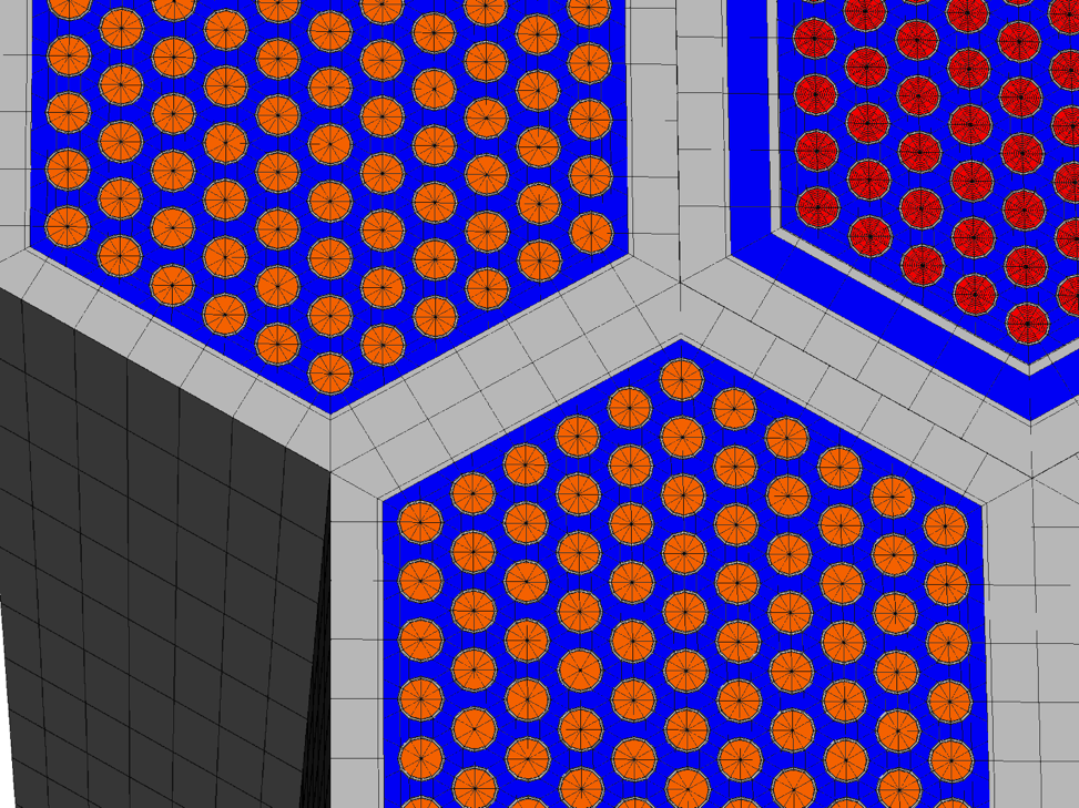
Figure 3.19.10 Pseudo Color Plot of Steady-State Coolant, Structure, and Fuel Temperatures (°C) for XX09 and Surrounding Assemblies.

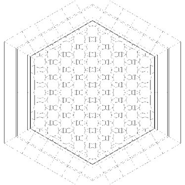
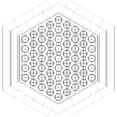
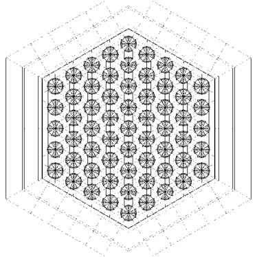
Because of the potential for the enormous amounts of data that need to be generated in order to fill a visualization mesh, an option is provided to control the level of detail represented in the visualization mesh geometry file on an assembly-by-assembly basis. Figure 3.19.10 displays two of the many detail options available. In Figure 3.19.10, experimental assembly XX09 is represented by a detailed radial pin mesh that includes nine radial temperature zones in the fuel region. The surrounding assemblies, however, are represented by an average fuel region that includes only a single radial zone for the bulk average fuel temperature. This reduces the data file for the 250 second simulation from the 15 GB estimate described earlier down to approximately 3.5 GB. The different options for the level of detail in the visualization mesh geometry file are listed in Table 3.19.19 and examples of the mesh for each option are shown in Table 3.19.20.

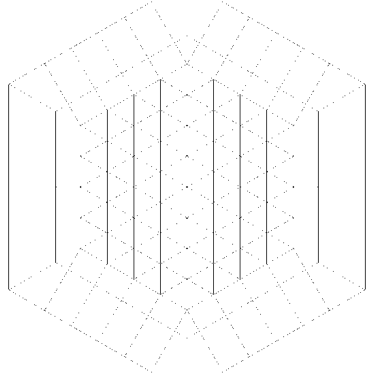
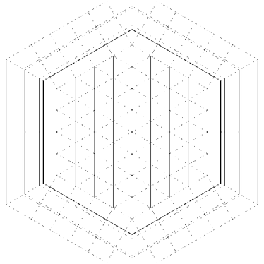
The detail options shown in Table 3.19.20 include two very simplified subchannel representations that use a single cell volume for each subchannel (LDETL = -1 or -2). For the interior subchannels, triangular cells are defined; and for the edge and corner subchannels, quadrilateral cells are defined. For LDETL = -1, these cells (artificially) extend over the fuel pin and structure regions in order to occupy the full assembly volume. For LDETL = -2, the cells only extend over the fuel pin regions, and additional cells are defined to represent the duct wall structure regions.

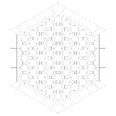
Positive values of LDETL define multiple coolant cells to approximate the actual shape of the coolant subchannel. LDETL = 1 and LDETL = 2 have void regions in the geometry since neither define regions for fuel pins and the former does not define regions for the duct wall structure. The advantage of LDETL = 1 and LDETL = 2 is that they require the same data as with the corresponding negative values for LDETL but they more accurately represent the physical geometry. LDETL options 3 and 4 introduce regions defined for the fuel pin, including fuel and cladding. The difference between the two options is that LDETL = 3 represents the fuel region by a single radial zone, while LDETL = 4 represents the fuel region by multiple radial zones corresponding to the parameter NT. (See below.)

Table 3.19.19 Geometry Detail Options for Creating Visualization Mesh Geometry Files.

Geometric Detail Option (LDETL Parameter)	Geometric Detail
0	No Geometry Defined
-1	Simplified Coolant Subchannels
-2	Simplified Coolant Subchannels and Duct Wall Structure
1	Detailed Coolant Subchannels
2	Detailed Coolant Subchannels and Duct Wall Structure
3	Detailed Coolant Subchannels, Duct Wall Structure, and Simplified Fuel Pin
4	Detailed Coolant Subchannels, Duct Wall Structure, and Detailed Fuel Pin

Table 3.19.20 Examples of Geometry Detail Options Applied to the XX09 Experimental Assembly.

LDETL = -1	LDETL = -2
LDETL = 1	LDETL = 2
LDETL = 3	LDETL = 4

It should be noted that even though the coolant subchannels are defined by multiple cells for positive values of LDETL (four in the case of the interior subchannels) SAS4A/SASSYS‑1 still only calculates a single temperature for each axial position along a subchannel and that temperature is applied to all cells that belong to a given subchannel. Therefore, it is important to recognize the distinction between the visualization mesh described here and the computation mesh (i.e. channel model) used by the SAS4A/SASSYS‑1 code.

In the multiple-pin subchannel preprocessor, all new parameters associated with the generation of a visualization mesh geometry file are confined to the assembly type definition input. This includes the geometric detail option parameter LDETL. Therefore, even if two assemblies are of the same type (both driver assemblies, for example) different types will need to be defined if a different level of geometric detail is desired for each. In the modified preprocessor, the additional parameters are expected only if the existing parameter IHEXP2 = 2. This assures compatibility with existing input files created for earlier versions of the preprocessor. When IHEXP2 = 2, the additional visualization input, shown in Section 3.19.2.3.3, must be added to the end of each assembly type definition.

Using the geometry information contained in the preprocessor input file, along with the additional visualization input shown in Section 3.19.2.3.3, the multiple-pin subchannel preprocessor can create a SAS4A/SASSYS‑1 visualization mesh geometry file. By default, the generated file is named “SAS.sasgeom”. Although the basename of the file is not critical, the file extension (*.sasgeom) is used by the VisIt visualization software to identify the correct file reader with which to parse the mesh.

The VisIt visualization software can be used to view the visualization mesh geometry file created by the preprocessor without needing to carry out a simulation to generate data. VisIt has the capability to plot numerous qualities of the visualization mesh, including determining individual cell volumes. In addition to the visualization mesh geometry, the file contains two parameters that can be plotted: channel ID and channel type. Channel ID directly corresponds to the SAS4A/SASSYS‑1 channel number, and can be used to identify specific channels in the global geometry. Channel type is somewhat of a misnomer, 7 in that it does not define a type for a given channel but rather a region to which a cell in the channel’s geometry belongs. (Figure 3.19.10 was created by plotting the channel type parameter.) The currently defined types include

• 0: Coolant (always present)

• 1-3: Cladding Radial Components (Inner, Middle, Outer; present when

  LDETL ≥ 3)

• 4-5: Structure Components (Inner, Outer; present when |LDETL| ≥ 2)

• 10: Bulk Fuel (present when LDETL = 3)

• 11-(10+NT): Radial Fuel Components (present when LDETL = 4)

Data generated during a simulation is associated with a cell in the visualization mesh by matching three parameters: channel ID, axial position, and channel type. This data can then further vary as a function of time. The creation of a SAS4A/SASSYS‑1 visualization data file is described in the following section.

3.19.3.3. Data Generation

The visualization capabilities introduced into SAS4A/SASSYS‑1 assume that geometry is invariant. This significantly simplifies implementation since the SAS4A/SASSYS‑1 code has limited knowledge of the specific geometric details needed to project computed simulation data into three-dimensional space. As described in the previous section, a visualization mesh geometry file is created by the multiple-pin subchannel preprocessor. Modifications have been made to the SAS4A/SASSYS‑1 code to produce a separate visualization data file that contains time-dependent simulation data that can be associated with the visualization mesh geometry. Details on the format of the visualization data file are contained in Section 3.19.3.7.

Two parameters have been added to the SAS4A/SASSYS‑1 input description to control the creation of the visualization data file. These two parameters are defined in Table 3.19.21. The first parameter, IVIS3D, indicates how often to write simulation data to the visualization data file. By default, the file created will be named “SAS.sasdata”. Like with the visualization mesh geometry file, the basename of the file is not critical, but the file extension (*.sasdata) is used by the VisIt visualization software to identify the correct file reader with which to parse the data file.

The second parameter, LDETL, is a channel-dependent parameter that controls the extent of data written for each channel. It corresponds to the LDETL parameter defined for the multiple-pin subchannel input preprocessor. When creating channel-dependent input using the input preprocessor, the LDETL parameter will automatically be written to the generated input description. Therefore, a user does not normally need to set this input parameter.

Table 3.19.21 SAS4A/SASSYS‑1 Input Parameters for Generation of Visualization Data

Parameter	Description
IVIS3D	Visualization Data Generation Flag: = 0, Do not write visualization data > 0, Write visualization data every IVIS3D time steps.
LDETL	Visualization Data Detail Flag: = 0, Do not write visualization data for this channel = 1, Write coolant temperatures only = 2, Coolant and duct wall temperatures = 3, Coolant, structure, and average fuel temperatures = 4, Coolant, structure, average fuel, and detailed radial fuel temperatures.

There are two minor differences in the treatment of the LDETL parameter between the multiple-pin subchannel input preprocessor and the SAS4A/SASSYS‑1 code. The input preprocessor allows negative values for LDETL, which correspond to coolant subchannel cells that completely occupy the assembly dimensions. However, the data needed for these two options is identical to the data needed for positive values of LDETL that have the same magnitude. Therefore, SAS4A/SASSYS‑1 only defines positive values for LDETL. The second difference is that for LDETL = 4, SAS4A/SASSYS‑1 also writes out the average fuel temperatures (corresponding to LDETL = 3) in addition to the detailed radial fuel temperatures. This is not done for the visualization mesh because it would define multiple cells for the same physical region. By writing this additional data, a visualization data file created as part of a simulation with LDETL = 4 can be used with a visualization mesh geometry file created with LDETL = 3 without having to re-run the simulation. In fact, once a visualization data file is created, it can be combined with a visualization mesh geometry file with a lower-magnitude LDETL parameter.

3.19.3.4. Data Visualization

The preceding sections describe the two-step process needed to create a visualization mesh geometry file and a visualization data file respectively. Interactively viewing the results of a simulation contained in these files is accomplished using the VisIt visualization software package freely available from Lawrence Livermore National Laboratory. VisIt is available for multiple computing platforms, including Linux, Windows, Mac OS X, Solaris, and others. In collaboration with LLNL, a Windows-based file reader plug-in for VisIt has been written that can parse the two files described here and import data into VisIt.

Each of the two files requires a unique file extension (*.sasgeom and *.sasdata) that VisIt uses to identify the correct file-reader plug-in to use when reading the data files. While the geometry file can be viewed independently of the data file, the data file requires a matching geometry file so that data can be projected into three-dimensional space. The matching of the geometry and data files is done by comparing a file’s basename. Therefore, SAS.sasdata will be associated with SAS.sasgeom (and vice versa). This process is handled automatically by the file reader.

VisIt supports extensive data visualization capabilities, including pseudo color plots, slices, contours, and animations as well as data picks (queries), filters, time derivatives, and the construction of arbitrary expressions based on existing data. The use of the VisIt visualization tool is beyond the scope of this memo. Details on downloading and using VisIt are currently found at http://www.llnl.gov/visit/.

To illustrate some of the visualization capabilities, two (static) examples from the SHRT-17 simulation are shown in Figure 3.19.11 and Figure 3.19.12. Figure 3.19.11 shows a plot of the XX09 assembly and its neighbors at t = 0 (steady state). The plot has been cropped through the center of XX09 to show the interior detail of fuel-pin temperatures. Figure 3.19.12 shows a contour plot of a slice at the top of the active core region at t = 90 seconds into the transient. Animated versions of both of these plots are presently archived at http://internal.ne.anl.gov/~fanning/SHRT17.html.

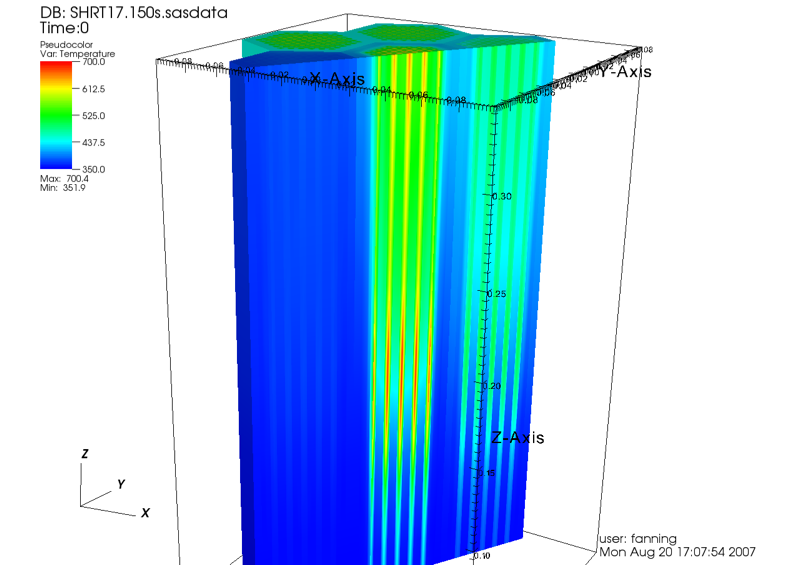
Figure 3.19.11 Pseudo Color Plot of Steady-State Coolant, Structure, and Fuel Temperatures (°C) for XX09 and Surrounding Assemblies.

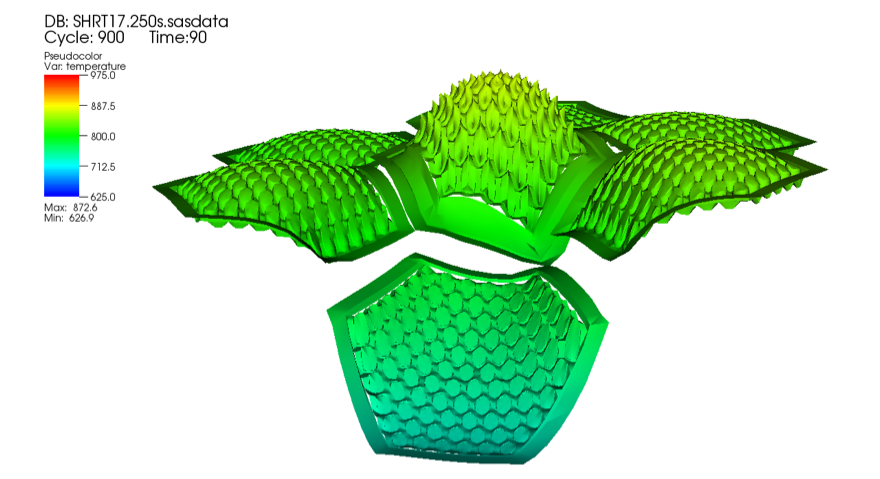
Figure 3.19.12 Contour Plot of Coolant, Structure, and Fuel Temperatures (°K) for XX09 and Adjacent Assemblies. (Top of Core at \(t = 90\) seconds)

3.19.3.5. Summary

An advanced visualization capability has been developed for the SAS4A/SASSYS‑1 code that allows for the generation, display, and animation of large datasets that are calculated during a transient simulation. The key features of the new capability include its support for multiple-pin, subchannel modeling, integration with the subchannel input preprocessor, geometry visualization, fully-detailed temperature field support with unlimited dataset sizes, and interactive visualization and animation generation on a desktop PC using the visualization tool VisIt.

3.19.3.6. References

1. J. E. Cahalan, et al., “Advanced LMR Safety Analysis Capabilities in the SASSYS-1 and SAS4A Computer Codes,” Proc. Int’l Topical Meeting on Advanced Reactor Safety, American Nuclear Society, Pittsburgh, PA, April 17-21, 1994.

2. “VisIt User’s Manual”, UCRL-SM-220449, Lawrence Livermore National Laboratory, October 2005.

3. F. E. Dunn, et al., “Whole Core Subchannel Analysis Verification with the EBR-II SHRT-17 Test,” Proc. ICAPP 2006, Reno NV, June 4-8, 2006.

3.19.3.7. File Formats

3.19.3.7.1. Visualization Mesh Geometry File

The visualization mesh geometry file is an unformatted (binary) Fortran file that contains a file header followed by two data sections. The first data section defines assembly types in a local coordinate system. The second data section defines actual assemblies in the problem geometry in terms of previously-defined types and offsets into a global coordinate system. This arrangement very much mimics the definition of assembly types and positions in the multiple-pin subchannel preprocessor. All numeric data is represented by four byte integers and double-precision (eight-byte) floating point values. Byte order does not matter, since the file reader for VisIt was designed to detect and support both conventions. However byte order must be consistent within a single file.

3.19.3.7.1.1. File Header

The file header consists of two records that identify file attributes and a problem title. The first record defines the following file attributes:

FILEID File ID. Must be the four characters SAS_. (The fourth character is a space.)

FILETYPE File Type. Must be the four characters GEOM.

GEOMVER1 Integer File Version. Currently, GEOMVER1 = 1.

GEOMVER2 Integer File Sub-version. Currently, GEOMVER2 = 0.

CHRDATE File Creation Date. (Eight-byte character string.)

CHRTIME File Creation Time. (Eight-byte character string.)

The first four attributes are used by the VisIt file reader to ensure that the correct reader is being used to parse the data file. If major or minor changes to the file format are introduced, the GEOMVER1 and GEOMVER2 attributes will be changed to identify the correct file format for the reader to parse.

The second record in the file header is an 80-character problem title. The multiple-pin subchannel preprocessor uses the problem title provided as input for this record.

3.19.3.7.1.2. Assembly Types

The first data section following the file header defines assembly types in a local coordinate system. Since most assemblies (for example, driver assemblies) will have the same geometry, this simplifies (and shortens) the overall visualization mesh geometry file.

The structure of the assembly type definitions is represented by the following pseudo code:

NTYPES

DO ITYPE = 1, NTYPES

  TYPE\_TITLE(ITYPE)

  ITYPEID(ITYPE), NCHAN(ITYPE), NZ(ITYPE),
(Z(K,ITYPE),K=1,NZ(ITYPE))

  DO J = 1, NCHAN(ITYPE)

    IRELCH(J,ITYPE), NP(J,ITYPE),
(X(I,J,ITYPE),Y(I,J,ITYPE),I=1,NP(J,ITYPE))

  ENDDO

ENDDO

The assembly type definitions begin with a record containing a single integer parameter, NTYPES, defining the number of assembly types contained in this data section. Each of the assembly type definitions that follow contains a title record (TYPE_TITLE, 80 characters) and an attributes record containing the following parameters:

ITYPEID Unique identification number for this assembly type.

NCHAN Number of “data channels” defined for this assembly type.

NZ Number of axial segments boundaries. (Typically, NZ = MZ + 1.)

Z Z coordinates of the axial segment boundaries in the local coordinate system.

Following the assembly type attributes record is one record for each of the NCHAN data channels defined for an assembly type. The data channel record defines the attributes and geometric shape (in the x-y plane) of the data channel:

IRELCH Relative data channel identification number. (See ICHOFF below.)

NP Number of vertices in the polygon defining this data channel. (Presently, NP must be 3 or 4.)

X, Y (X,Y) coordinates of the vertices defining the polygon for this data channel in local coordinates.

3.19.3.7.1.3. Assembly Definitions

The second data section defines “actual” assemblies in the problem geometry by placing assembly types defined earlier into a global coordinate system. The structure of the assembly definitions is represented by the following pseudo code:

NSUBS

DO ISUB = 1, NSUBS

  SUB\_TITLE(ISUB)

  ISUBID(ISUB), ISUBTYPEID(ISUB), ICHOFF(ISUB),
XOFF(ISUB),YOFF(ISUB),ZOFF(ISUB)

ENDDO

The subassembly definitions begin with a record containing a single integer parameter, NSUBS, defining the number of assemblies being specified in the visualization mesh geometry file. This need not represent all the assemblies in the problem geometry, only those for which a visualization mesh is needed. Each of the assembly definitions that follow contains a title record (SUB_TITLE, 80 characters) and an assembly attributes record containing the following parameters:

ISUBID Identification number for this subassembly.

ISUBTYPEID Identification number of the assembly type being used to define this assembly.

ICHOFF Integer offset to translate each relative data channel identification number into an absolute (global) data channel identification number.

XOFF, YOFF, ZOFF Coordinate offsets to translate local coordinates of the type definition into global coordinates of the problem geometry.

Absolute data channel identification numbers are constructed from the sum of the relative data channel identification number (IRELCH) and the data channel offset (ICHOFF) for each of the data channels that define an assembly type. For data channels that represent coolant, IRELCH typically starts at 1 and increases by 1 for each coolant subchannel in the assembly type definition. When added to ICHOFF, the resulting data channel identification corresponds to the channel number (ICH) in the SAS4A/SASSYS‑1 simulation. Note that because multiple data channels may be used to represent the complex shape of a particular region (the coolant region of a subchannel, for example) absolute data channel identification numbers need not be unique in the visualization mesh geometry file.

For data channels that represent regions other than coolant, an additional term is introduced into the definition of IRELCH. If ICHTYPE represents the channel types as defined by the bulleted list on Page 3-184, then the additional term added to IRELCH is equal to ICHTYPE×10⁶. This procedure is also used by SAS4A/SASSYS‑1 to create data channel identification numbers based on the channel number, ICH, and guarantees correct association between the visualization mesh and the simulation data. That is, simulation data is correctly associated with the visualization mesh when (IRELCH + ICHOFF) = (ICHTYPE×10⁶ + ICH).

3.19.3.7.2. Visualization Data File

The visualization data file is an unformatted (binary) Fortran file that contains a file header followed by one data section for each time step saved during a simulation. All numeric data is represented by four byte integers and double-precision (eight-byte) floating point values. Byte order does not matter, since the file reader for VisIt was designed to detect and support both conventions. However byte order must be consistent within a single file.

3.19.3.7.2.1. File Header

The simulation data file header consists of a record that identifies file attributes and two problem title records. The first record defines the following file attributes:

FILEID File ID. Must be the four characters SAS_. (The fourth character is a space.)

FILETYPE File Type. Must be the four characters DATA.

DATAVER1 Integer File Version. Currently, DATAVER1 = 1.

DATAVER2 Integer File Sub-version. Currently, DATAVER2 = 0.

CHRDATE File Creation Date. (Eight-byte character string.)

CHRTIME File Creation Time. (Eight-byte character string.)

The first four attributes are used by the VisIt file reader to ensure that the correct reader is being used to parse the data file. If major or minor changes to the file format are introduced, the DATAVER1 and DATAVER2 attributes will be changed to identify the correct file format for the reader to parse.

The second and third records in the file header represent two 80-character problem titles. The problem titles are determined by the two title records provided as part of the SAS4A/SASSYS‑1 input.

3.19.3.7.2.2. Simulation Data

The remainder of the visualization data file consists of repeated blocks of simulation data. Data blocks contain simulation data for each time step that is recorded as determined by the value of the IVIS3D input parameter. The details of the simulation data that is recorded are determined by the channel-dependent input parameter, LDETL. The arrangement of data in the simulation data block is described by the following pseudo code:

TIME, NDATA

DO J = 1, NDATA

  ICHID(J), ND(J), (DATA(J,K),K=1,ND)

ENDDO

The first record in the data block contains the current simulation time (TIME) and the number of data channels that are to follow (NDATA). Although all data blocks from a simulation will have the same length and the same number of data channels, the NDATA parameter is provided to facilitate parsing and verification by file readers.

Following the initial record is a series of NDATA records containing simulation data represented by the following parameters:

ICHID Unique ID for this data channel.

ND Number of axial data values for this data channel. (Typically, ND = MZ.)

DATA Simulation data, with one value for each axial position.

Data channel IDs must be unique within each data block and are associated with zero or more data channels in the visualization mesh geometry in order to project the data into three-dimensional space. The construction of the data channel ID is described in the previous section as \(\text{ICHID} = \left( \text{ICHTYPE} \times 10^{6} + \text{ICH} \right)\) and ensures a unique value based on SAS4A/SASSYS‑1 channel numbers (ICH) and the type of data being stored.

1

A row of pins is the same as a ring of pins

2

Equations reference other variable columns using the assigned letter. SC=Subchannel, SA=Subassembly.

3

Thimble flow region not shown

4

These parameters are only used to generate the visualization mesh geometry and, with the exception of LDETL, are not incorporated into the SAS4A/SASSYS‑1 input that is generated for the subchannel definitions.

5

SA = Subassembly

6

Animations of the SHRT-17 simulation can be viewed at http://internal.ne.anl.gov/~fanning/SHRT17.html

7

The misnomer arises because the channel ID and channel type parameters actually exist in the geometry file as a single integer parameter that represents a unique “data channel” that is used to associate simulation data with the visualization mesh.

3.19.4. APPENDIX 3.4: Coolant Physical Properties

3.19.4.1. Introduction

The expressions used in SAS4A/SASSYS-1 to model coolant physical properties as functions of temperature are derived from data correlations generated by Padilla [12.1] and by Fink and Leibowitz [12-12]. These correlations were developed using sodium coolant properties that match the most recent measurements available, namely those of Bhise and Bonilla [12-13] and Da Gupta and Bonilla [12-14]. The mathematical forms of these properties are maintained for coolants independent of their composition.

The mathematical expressions for coolant physical properties are provided in the sections below, including brief descriptions of their origins. In all cases, the temperature \(T\) is in Kelvin.

3.19.4.2. Sodium Coolant Physical Properties

Details for sodium coolant properties and the associated polynomial coefficients are described in Section 12.13. This information is not repeated here.

3.19.4.3. Lead Coolant Physical Properties

The lead coolant properties are derived from the data and correlations available in [A3.4-1]. The mathematical expressions in [A3.4-1] are not directly implemented, but rather a least-squares approximation to these correlations was generated for lead coolant properties to match the existing sodium-derived forms implemented within SAS4A/SASSYS-1. The error introduced by this approach, which is largely considered negligible, has been quantified and documented in the sections below.

3.19.4.3.1. Lead Critical Temperature

The critical temperature (T_c) is an important parameter for the development of an equation of state (EOS) and the extension of information on the available thermophysical data to higher temperatures and pressures. A very large uncertainty exists in the critical temperature for lead as indicated in [A3.4-1].

The literature review performed in [A3.4-1] takes into account the large uncertainty in the estimations of the critical temperature. The value recommended is:

(A3.4‑1)

\[\text{T}_{Crit} = 5000.0 \pm 200 \text{ K}\]

3.19.4.3.2. Lead Heat of Vaporization

The heat of vaporization at the normal boiling point is also referred to the latent heat (enthalpy) of vaporization in the literature. It quantifies the energy required to break the atomic binding in lead.

The literature review in [A3.4-1] outlines a relatively small standard deviation. The recommended value in [A3.4-1] for the latent heat of vaporization for pure lead at the normal boiling point is:

(A3.4‑2)

\[\text{Q} = 858.6 \pm 1.9 \text{ kJ/kg}\]

The heat of vaporization correlation implemented in SAS4A/SASSYS-1 uses a temperature-dependent polynomial to compute this quantity:

(A3.4‑3)

\[\lambda = A_1 + A_2 T + A_3 T^{2} + A_4 T^{3}\]

Lead’s latent heat is a constant and, therefore, only \({A}_{1}\) is specified. The corresponding values for the coefficients of Eq. A3.4-3 are provided in Section 3.19.4.6.

3.19.4.3.3. Lead Saturation Pressure

The lead saturation pressure as a function of temperature is an important property of coolants. It determines the dependence of the boiling temperature on pressure and heat-mass transfer in the cover gas space. It is directly related to the latent heat (enthalpy) of vaporization. [A3.4-1] provides two correlations for the saturation pressure. The expression chosen for the latent heat of vaporization for pure lead at the normal boiling point is:

(A3.4‑4)

\[P_{S} = 1.88 × 10^{13} T^{-0.985} e^{\left ( \frac{-23325}{T} \right )}\]

The saturated vapor pressure is defined within a temperature range of \([\text{T}_{M,0(Pb)}-\text{T}_{B,0(Pb)} ]\) where \(\text{T}_{M,0(Pb)}\) represents the normal melting point \((600.6\text{ K})\) and \(\text{T}_{B,0(Pb)}\) is the normal boiling point \((2021 \pm 3 \text{ K})\). Per [A3.4-1], the standard deviation with respect to the data is:

• 15% for temperatures within the range \([\text{T}_{M,0(Pb)} - 1100\text{ K}]\)

• 5% for temperatures within the range \([1100\text{ K} - \text{T}_{B,0(Pb)}]\)

The calculation of the saturation pressure in SAS4A/SASSYS-1 correlates the natural logarithm of the saturation pressure to a temperature-dependent polynomial.

(A3.4‑5)

\[ln(P_{S}) = A_5 - \frac{A_6}{T} - \frac{A_7}{T^2}\]

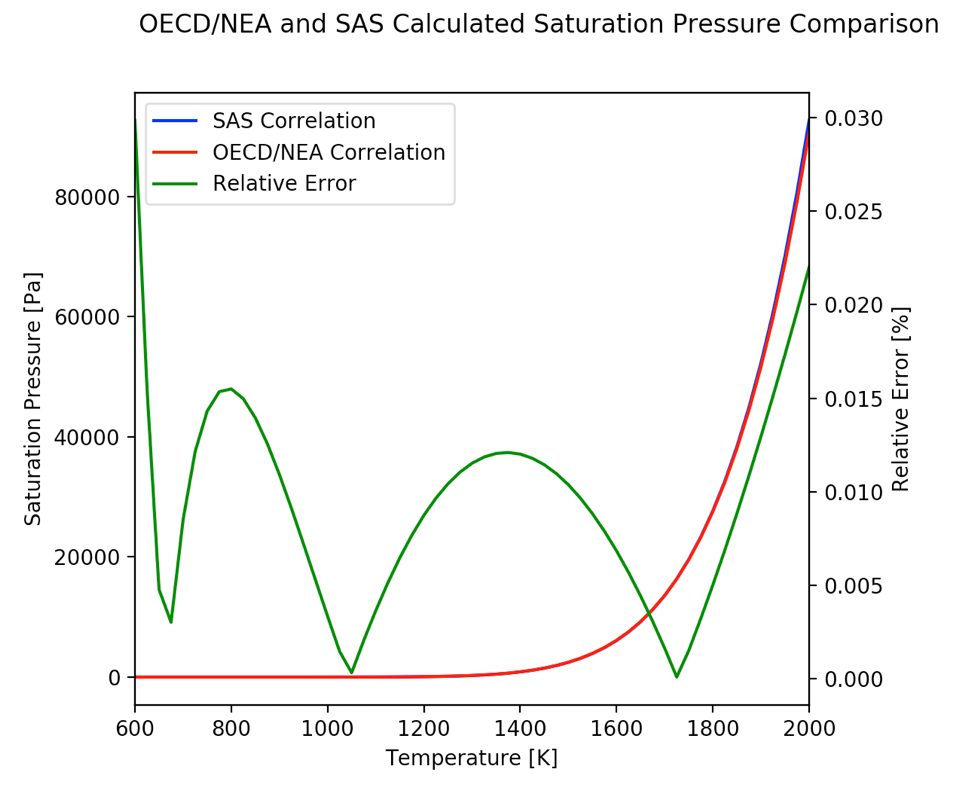
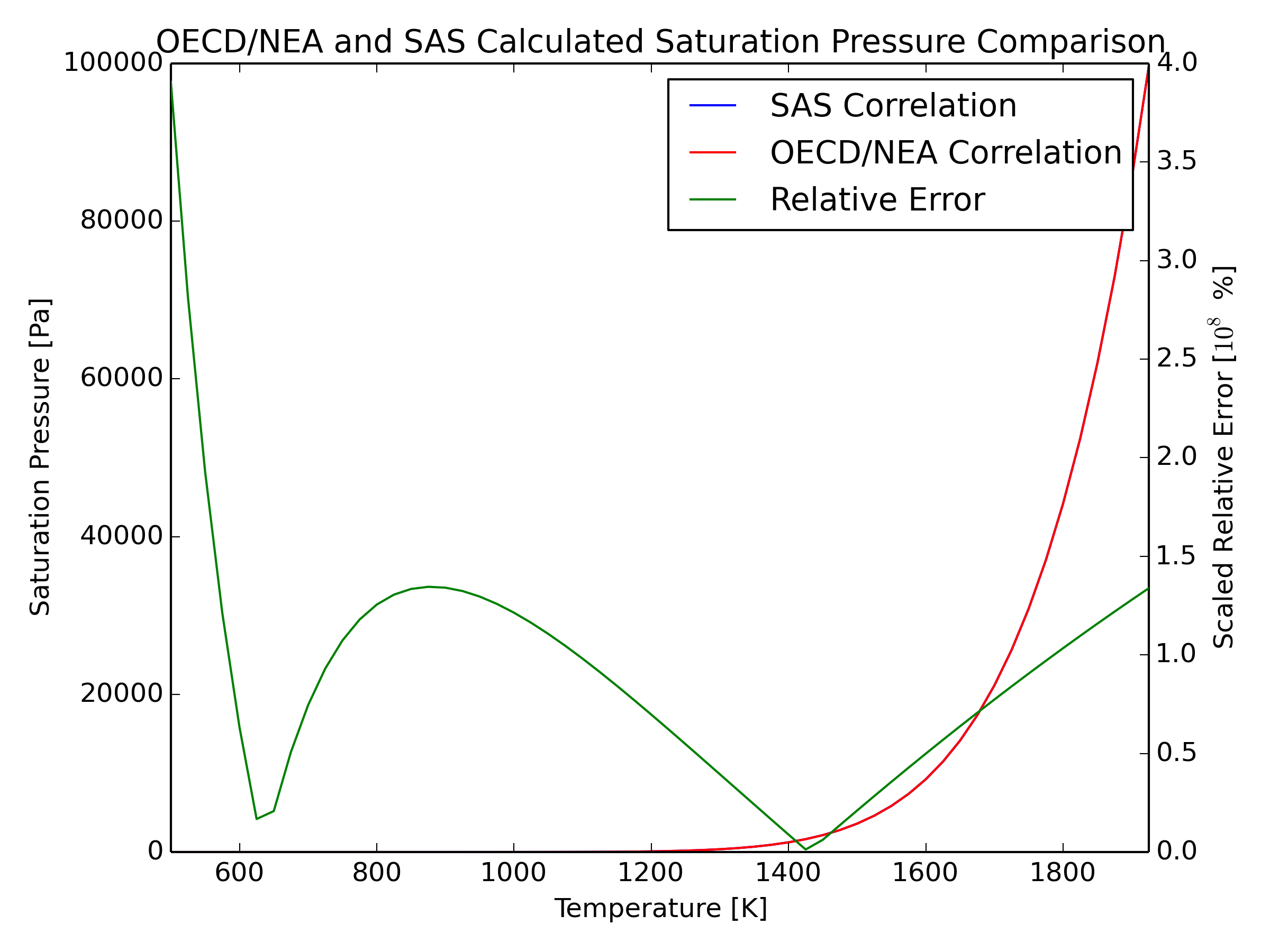
The constant coefficients in the SAS4A/SASSYS-1 second order correlation were evaluated using a least squares equal weighted residual minimization fit to the OECD compressibility correlation. The corresponding values for the coefficients of Eq. A3.4-5 are provided in Section 3.19.4.6.

The temperature range provided in [A3.4-1] was maintained when performing the least square fit to adapt to the form of Eq. A3.4-5. Uncertainties for this correlation are not determined. However, absolute and relative errors with respect to the OECD correlation were calculated. The relative error is provided in the plot below.

3.19.4.3.4. Lead Saturation Temperature

SAS4A/SASSYS-1 requires an expression for temperature as a function of pressure. This expression is obtained by inverting Eq. A3.4-5. Direct inversion yields:

(A3.4‑6)

\[T_{S} = \frac{A_8}{A_9+\sqrt{A_{10}+A_{11}ln \left( P_S\right)}}\]

The corresponding values for the coefficients of Eq. A3.4-6 are provided in Section 3.19.4.6.

3.19.4.3.5. Lead Liquid Density

The lead density depends on temperature and pressure. The expression recommended in [A3.4-1] for the lead density defines a linear temperature dependence of the form:

(A3.4‑7)

\[\rho_{l} = 11441 - 1.2795 T\]

The accuracy with which this correlation reproduces selected literature sources is discussed in [A3.4-1]. The maximum difference does not exceed 1% within the temperature range from the normal melting point \(\text{T}_{M,0(Pb)}\) to \(1500 \text{ K}\). This difference becomes about 2% when temperature increases up to the normal boiling point (defined as \(\text{T}_{B,0(Pb)} = 2021 \pm 3 \text{ K}\)).

The SAS4A/SASSYS-1 mathematical expression correlating the coolant density to the temperature is a second order polynomial:

(A3.4‑8)

\[\rho_{l} = A_{12} + A_{13} T + A_{14} T^2\]

The corresponding values for the coefficients of Eq. A3.4-8 are provided in Section 3.19.4.6. The correlation accuracy and temperature range of [A3.4-1] is consistent with Eq. A3.4-8 since the correlation mathematical form is maintained.

3.19.4.3.6. Lead Vapor Density

Discussion of lead vapor density is not available in [A3.4-1], and alternative literature/experimental sources are not widely available.

The calculation of the vapor density in SAS4A/SASSYS-1 uses a temperature-dependent polynomial which is multiplied by the saturation temperature:

(A3.4‑9)

\[\rho_{v} = P_{S} \left ( \frac{A_{15}}{T} + A_{16} + A_{17} T + A_{18} T^2 + A_{19} T^3 + A_{20} T^4 \right )\]

The corresponding values for the coefficients of Eq. A3.4-9 are provided in Section 3.19.4.6. For the current implementation, a value for \(A_{15} = 0.01\) is assumed, and all other coefficients are assumed to be zero. The temperature range over which this correlation is applicable is unknown, but it is assumed that it applies to temperatures above \(\text{T}_{B,0(Pb)} = 2021 \pm 3 \text{ K}\) where lead vapor is anticipated to be present.

3.19.4.3.7. Lead Liquid Specific Heat

Calculation of the coolant enthalpy change as a function of temperature requires knowledge of the isobaric heat capacity. To account for large uncertainties in the data, [A3.4-1] proposes the following expression for liquid lead specific heat:

(A3.4‑10)

\[C_{l} = 176.2 - 4.923× 10^{-2} T + 1.544×10^{-5} T^2 - \frac{1.524×10^{6}}{T^2}\]

[A3.4-1] identifies a 1991 correlation, which was later refined, as a reasonable choice for the isobaric heat capacity of pure liquid lead in the temperature range of \([\text{T}_{B,0(Pb)} - 2000 \text{ K}]\). The accuracy with which this refined correlation reproduces selected literature sources is discussed in [A3.4-1]. The estimated uncertainty is 5-7% within \([\text{T}_{B,0(Pb)} - 1500 \text{ K}]\) and 7-15% at higher temperatures where no experimental data is available in literature.

In SAS4A/SASSYS-1, the liquid specific heat is approximated by a polynomial that considers the difference between coolant temperature and critical temperature (Eq. A3.4-1):

(A3.4‑11)

\[C_{l} = \frac{A_{28}}{\left( T_{C} - T \right)^2} + \frac{A_{29}}{\left( T_{C} - T \right)} + A_{30} + A_{31} (T_{C} - T) + A_{32} \left ( T_{C} - T \right )^{2}\]

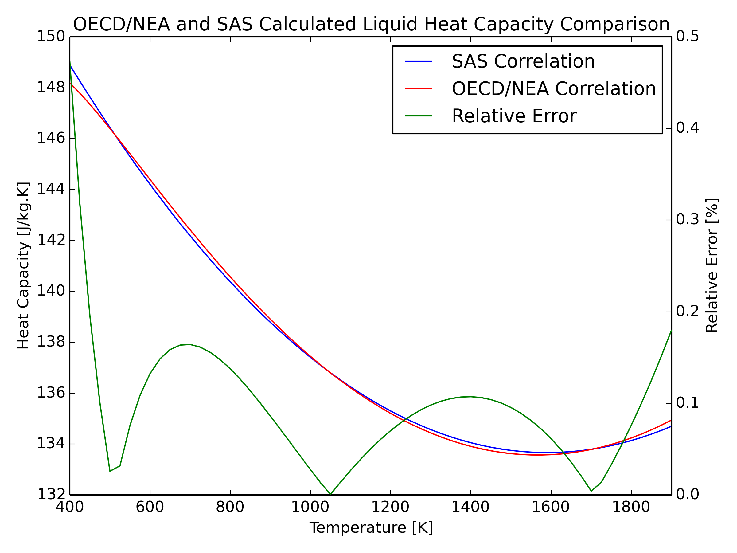
The mathematical expressions in [A3.4-1] and that of SAS4A/SASSYS-1 have different forms. The constant coefficients in the SAS4A/SASSYS-1 correlation were evaluated using a least squares equal weighted residual minimization fit to the [A3.4-1] specific heat correlation. The temperature range over which this correlation was determined in [A3.4-1] is maintained as the least square fit to Eq. A3.4-11 was applied over the range outlined above. The corresponding values for the coefficients of Eq. A3.4-11 are provided in Section 3.19.4.6.

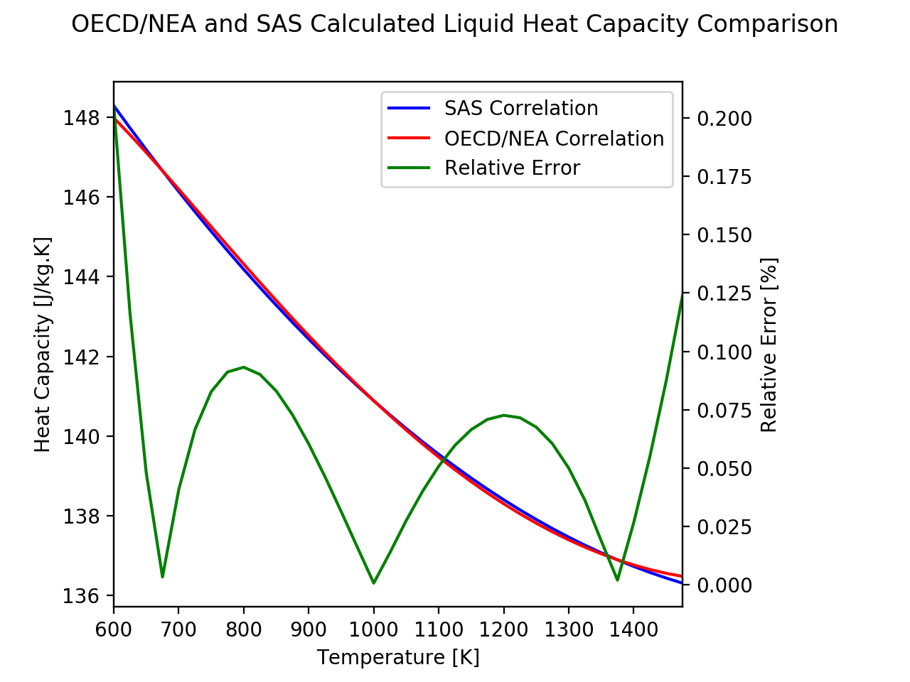
Absolute and relative errors with respect to the OECD correlation were calculated, with relative error provided in the plot below.

3.19.4.3.8. Lead Vapor Specific Heat

Reference [A3.4-1] does not discuss vapor specific heat. No experimental data related to the specific heat of lead vapor could be found.

Lead boiling is not expected to occur within the temperature ranges typically considered for lead fast reactors in the design basis analysis envelope. Moreover, in the unlikely event that lead boiling were to occur, this phenomenon will likely be localized for these particular scenarios. Due to the lack of literature on this subject, its limited relevance the typical SAS4A/SASSYS-1 analysis scope, and unavailability of a two-phase lead coolant model in SAS4A/SASSYS-1, vapor specific heat is ignored. The corresponding values for the related coefficients are provided in Section 3.19.4.6.

It should be noted that this assumption is not applicable for severe accidents where coolant boiling occurs at a larger scale.

3.19.4.3.9. Lead Adiabatic Compressibility

Reference [A3.4-1] assumes compressibility is a reversible adiabatic process. As such, the isentropic compressibility of the coolant at normal pressure is calculated as the inverse of the bulk elastic modulus. The bulk elastic modulus discussed in [A3.4-1] uses a polynomial as a function of temperature. As such, the expression for the compressibility becomes:

(A3.4‑12)

\[\beta_{s} = \left( \left( 43.50 - 1.552×10^{-2}T + 1.622×10^{-6}T^2 \right) × 10^{9} \right)^{-1}\]

The accuracy with which this correlation predicts compressibility is not directly discussed in [A3.4-1]. The report outlines how both compressibility and sound velocity are basic thermodynamic properties of molten lead. The Dreyfus thermodynamic relationship is used to infer the sound celerity from the bulk elastic modulus, and compressibility. Per [A3.4-1], the correlation is applicable for sound celerity of the longitudinal sound waves in molten lead for temperatures up to 1400K (i.e. \([\text{T}_{M,0(Pb)} - 1400 \text{ K}]\)). This range is assumed to be the same for compressibility.

The compressibility coefficient is calculated in SAS4A/SASSYS-1 by a polynomial expression based on the inverse of the coolant temperature subtracted from the critical temperature Eq. A3.4-1).

(A3.4‑13)

\[\beta_{s} = A_{40} + \frac{A_{41}}{\left( T_{C} - T \right)}\]

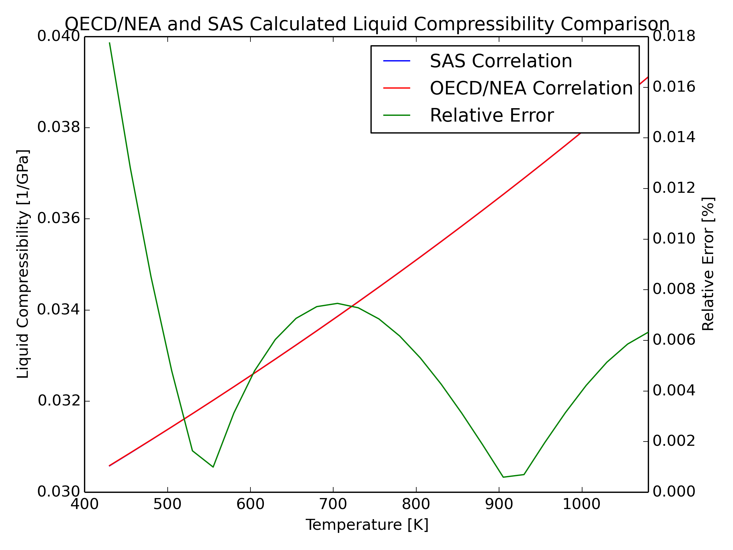
The mathematical expressions in [A3.4-1] and SAS4A/SASSYS-1 have different forms. The constant coefficients in the SAS4A/SASSYS-1 correlation were evaluated using a least squares equal weighted residual minimization fit to Eq. A3.4-12. The corresponding values for the coefficients of Eq. A3.4-13 are provided in Section 3.19.4.6.

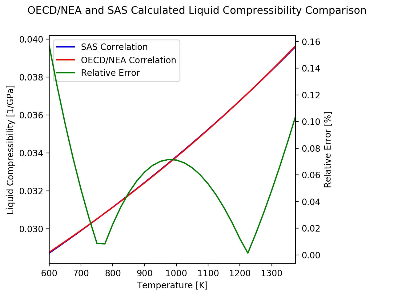
Uncertainties for this correlation were not determined. However, absolute and relative errors with respect to Eq. A3.4-12 were calculated. The relative error is provided in the plot below.

3.19.4.3.10. Lead Thermal Expansion

The density of liquid metals changes with temperature due to thermal expansion related to anharmonicity of interatomic forces. As outlined in [A3.4-1], the relationship between the density and the coefficient of volumetric thermal expansion (CVTE) at constant pressure \(p\) is defined by the following formula:

(A3.4‑14)

\[\alpha_{p} = -\frac{1}{\rho} \left ( \frac{\partial \rho}{\partial T} \right )_{p}\]

Substituting the correlations for density recommended by [A3.4-1] yields:

(A3.4‑15)

\[\alpha_{p} = \frac{1}{8942-T}\]

Since the thermal expansion correlation is defined from that of the density, the same temperature range of \([\text{T}_{M,0(Pb)} - 1400 \text{ K}]\)) applies. The uncertainty of this quantity can be derived from the thermal expansion expression and the coolant density uncertainty.

The thermal expansion coefficient is calculated in SAS4A/SASSYS-1 by a polynomial expression based on the inverse of the coolant temperature subtracted to the critical temperature:

(A3.4‑16)

\[\alpha_{p} = A_{42} + \frac{A_{43}}{\left( T_{C} - T \right)} + \frac{A_{44}}{\left( T_{C} - T \right)^2} + \frac{A_{45}}{\left( T_{C} - T \right)^3} + \frac{A_{46}}{\left( T_{C} - T \right)^4} + \frac{A_{47}}{\left( T_{C} - T \right)^5}\]

A simple polynomial form matching between equations in Eq. A3.4-15 and Eq. A3.4‑16) does not allow the SAS4A/SASSYS-1 expression to match that of [A3.4-1] with a reasonably small variation. Therefore, additional terms had to be included in the SAS4A/SASSYS-1 correlation. The correlation implemented includes terms from Eq. A3.4‑16) up to the third order. The constant coefficients in the SAS4A/SASSYS-1 correlation were evaluated using a least squares equal weighted residual minimization fit to the OECD thermal expansion correlation. The corresponding values for the coefficients of Eq. A3.4-16 are provided in Section 3.19.4.6.

Uncertainties for this correlation were not determined. However, absolute and relative errors with respect to Eq. A3.4-15 were calculated. The relative error is provided in the plot below.

3.19.4.3.11. Lead Thermal Conductivity

Thermal conductivity is the fundamental thermophysical parameter of liquid metal coolants, which is used in all heat transfer calculations. The accuracy of its determination for liquid metals is poor and usually large discrepancies exist among different sets of data. Per [A3.4-1], the following linear correlation was used as the thermal conductivity of the technically pure liquid lead at normal pressure:

(A3.4‑17)

\[k_{l} = 9.2 + 0.011 T\]

The accuracy with which this correlation reproduces selected literature sources is discussed in [A3.4-1]. The correlation is applicable from the lead melting temperature at normal atmospheric pressure up to 1300K (i.e. \([\text{T}_{M,0(Pb)} - 1300 \text{ K}]\)) with an estimated standard deviation of 15%. The SAS4A/SASSYS-1 mathematical expression correlating the coolant density to the temperature is a third order polynomial as defined below:

(A3.4‑18)

\[k_{l} = A_{48} + A_{49} T + A_{50} T^2 + A_{51} T^3\]

The corresponding values for the coefficients of Eq. A3.4-18 are provided in Section 3.19.4.6. The correlation accuracy and temperature ranges of Eq. A3.4-17 and Eq. A3.4-18 are consistent since the mathematical correlation form is maintained.

3.19.4.3.12. Lead Viscosity

Viscosity is a measure of friction among atoms of liquids. Because there is very little data on the impact of impurities on viscosity, the correlations below are for pure lead. Lead is believed to be a Newtonian liquid. Therefore, the temperature dependence of their dynamic viscosity is usually described by an Arrhenius-type equation as described in [A3.4-1].

(A3.4‑19)

\[\mu_{l} = 4.55×10^{-4}e^{\left ( \frac{1069}{T}\right )}\]

This correlation is valid in the temperature range from \([\text{T}_{M,0(Pb)} - 1473 \text{ K}]\) with an estimated uncertainty of \(\pm 5%\). Coolant dynamic viscosity is calculated in SAS4A/SASSYS-1 by a polynomial expression based on the inverse of the coolant temperature.

(A3.4‑20)

\[\mu_{l} = A_{52} + \frac{A_{53}}{T} + \frac{A_{54}}{T^2} + \frac{A_{55}}{T^3}\]

The mathematical expressions in Eq. A3.4‑19 and Eq. A3.4‑20 have different forms. The constant coefficients in the SAS4A/SASSYS-1 correlation were evaluated using a least squares equal weighted residual minimization fit to the OECD viscosity correlation. The corresponding values for the coefficients of Eq. A3.4-20 are provided in Section 3.19.4.6.

The temperature range over which this correlation was determined in [A3.4-1] is maintained because the least square fit to Eq. A3.4-19 was performed over the applicability range outlined above. Uncertainties for this correlation were not determined. However, absolute and relative errors with respect to Eq. A3.4-19 were calculated. The relative error is provided in the plot below.

3.19.4.4. LBE Coolant Physical Properties

The LBE coolant properties are derived from the data and correlations available in [A3.4-1]. The mathematical expressions in [A3.4-1] are not directly implemented for some properties, but rather a least-squares approximation to these correlations was generated for coolant properties to match the existing sodium-derived forms implemented within SAS4A/SASSYS-1. The error introduced by this approach, which is largely considered negligible, has been quantified and documented in the sections below.

3.19.4.4.1. LBE Critical Temperature

The critical temperature (T_c) is an important parameter for the development of an equation of state (EOS) and the extension of information on the available thermophysical data to higher temperatures and pressures.

A very large uncertainty still exists in the critical temperature for LBE as indicated in [A3.4-1], as no measurement data is available in public literature. Critical parameters are only available through theoretical estimations. The literature review performed in [A3.4-1] takes into account the three available estimations of the critical temperature. The value recommended by [A3.4-1], bounded by the uncertainties of lead and bismuth, is:

(A3.4‑21)

\[\text{T}_{Crit} = 4800.0 \pm 500 \text{ K}\]

3.19.4.4.2. LBE Heat of Vaporization

The heat of vaporization at the normal boiling point is also referred to the latent heat (enthalpy) of vaporization in the literature. It quantifies the energy required to break the atomic binding in LBE. The literature review in [A3.4-1] indicates limited availability of information. The recommended value in [A3.4-1] for the latent heat of vaporization of pure LBE at the normal boiling point is:

(A3.4‑22)

\[\text{Q} = 856 \pm 5 \text{ kJ/kg}\]

The heat of vaporization correlation implemented in SAS4A/SASSYS-1 uses a temperature-dependent polynomial to compute this quantity:

(A3.4‑23)

\[\lambda = A_1 + A_2 T + A_3 T^{2} + A_4 T^{3}\]

The latent heat of LBE is a constant and, therefore, only \({A}_{1}\) is specified. The corresponding values for the coefficients of Eq. A3.4-23 are provided in Section 3.19.4.6.

3.19.4.4.3. LBE Saturation Pressure

Vapor pressure as a function of temperature is an important property of coolants. It determines the dependence of the boiling temperature on pressure and heat-mass transfer in the cover gas space. It is directly related to the latent heat (enthalpy) of vaporization. The expression recommended by [A3.4-1] for the saturation pressure for pure LBE is:

(A3.4‑24)

\[P_{S} = 1.22 × 10^{10} e^{\left ( \frac{-22552}{T} \right )}\]

The literature review in [A3.4-1] indicates very large uncertainties exist at low temperatures \(\left( < ~773 \text{K} \right)\). Experimental data used to develop the above correlation is defined within a temperature range of \([500 - 1943 \text{K}]\). The OECD correlation standard deviation with respect to the data is, per [A3.4-1]:

• \(\pm 60\text{%}\) for temperatures within the range \([673 - 1927 \text{K}]\), and

• No agreement below 673 K.

The calculation of the saturation pressure in SAS4A/SASSYS-1 correlates the natural logarithm of the saturation pressure to a temperature-dependent polynomial.

(A3.4‑25)

\[ln(P_{S}) = A_5 - \frac{A_6}{T} - \frac{A_7}{T^2}\]

The constant coefficients in the SAS4A/SASSYS-1 second order correlation were evaluated using a least squares equal weighted residual minimization fit to the OECD correlation. The corresponding values for the coefficients for saturation pressure are provided in Section 3.19.4.6.

The temperature range provided in [A3.4-1] was maintained when performing the least square fit to adapt to the form of Eq. A3.4-25. Uncertainties for this correlation are not determined. However, absolute and relative errors with respect to the OECD correlation were calculated. The relative error is provided in the plot below.

3.19.4.4.4. LBE Saturation Temperature

SAS4A/SASSYS-1 requires an expression for temperature as a function of pressure. This expression is obtained by inverting Eq. A3.4-25. Direct inversion yields:

(A3.4‑26)

\[T_{S} = \frac{A_8}{A_9+\sqrt{A_{10}+A_{11}ln \left( P_S\right)}}\]

The corresponding values for the coefficients of Eq. A3.4-26 are provided in Section 3.19.4.6.

3.19.4.4.5. LBE Liquid Density

The LBE density depends on temperature and pressure. The expression recommended in [A3.4-1] for the lead density defines a linear temperature dependence of the form:

The coolant density depends on temperature and pressure. This quantity is essential to the development of an EOS. The expression recommended for the LBE density defines a linear temperature dependence of the form [A3.4-1]:

(A3.4‑27)

\[\rho_{l} = 11065 - 1.293 T\]

The accuracy with which this correlation reproduces selected literature sources is discussed in [A3.4-1]. The maximum difference does not exceed 0.8% within the temperature range of \([673 - 1927 \text{K}]\).

The SAS4A/SASSYS-1 mathematical expression correlating the coolant density to the temperature is a second order polynomial:

(A3.4‑28)

\[\rho_{l} = A_{12} + A_{13} T + A_{14} T^2\]

The corresponding values for the coefficients of Eq. A3.4-28 are provided in Section 3.19.4.6. The correlation accuracy and temperature range of [A3.4-1] is consistent with Eq. A3.4-28 since the correlation mathematical form is maintained.

3.19.4.4.6. LBE Vapor Density

Reference [A3.4-1] does not discuss vapor density. No experimental data related to this property could be found. Boiling is not expected to occur within the temperature range anticipated for design basis accidents in LBE-cooled fast reactors. However, in the unlikely event that coolant boiling were to occur, this phenomenon will likely be localized. Because of degraded heat transfer to vapor form coolant, coolant vapor temperature is not expected to raise significantly above saturation temperature.

The calculation of the vapor density in SAS4A/SASSYS-1 uses a temperature-dependent polynomial which is multiplied by the saturation pressure:

(A3.4‑29)

\[\rho_{v} = P_{S} \left ( \frac{A_{15}}{T} + A_{16} + A_{17} T + A_{18} T^2 + A_{19} T^3 + A_{20} T^4 \right )\]

The corresponding values for the coefficients of Eq. A3.4-29 are provided in Section 3.19.4.6. For the current implementation, a value for \(A_{15} = 0.01\) is assumed, and all other coefficients are assumed to be zero. The temperature range over which this correlation is applicable is unknown, but it is assumed that it applies to temperatures above \(\text{T}_{B,0(LBE)} = 1927 \pm 16 \text{ K}\) where LBE vapor is anticipated to be present.

3.19.4.4.7. LBE Liquid Specific Heat

Heat capacity is one of the most important properties of a coolant. Calculation of the coolant enthalpy change as a function of temperature requires knowledge of the isobaric heat capacity.

Discussion in [A3.4-1] indicates a limited availability of independent data on liquid specific heat. Leveraging the similarity of Pb-Bi to its components, available experimental data, and Kopp’s law (typically used to derive heat capacities of binary systems), a single polynomial was developed in [A3.4-1]. As such, the expression for the molten coolant specific heat becomes:

(A3.4‑30)

\[C_{l} = 164.8 - 3.94× 10^{-2} T + 1.25×10^{-5} T^2 - \frac{4.56×10^{5}}{T^2}\]

The OECD correlation uncertainty with respect to the data is, per [A3.4-1]:

• < 5% for temperatures within the range \([400 – 1100 \text{K}]\), and

• 1 – 2% within the range \([1100 - \text{T}_{B,0(LBE)} = 1927 \pm 16 \text{K}\), where the validity of Kopp’s law is most effective.

In SAS4A/SASSYS-1, the liquid specific heat is approximated by a polynomial that considers the difference between coolant temperature and critical temperature (Eq. A3.4-1):

(A3.4‑31)

\[C_{l} = \frac{A_{28}}{\left( T_{C} - T \right)^2} + \frac{A_{29}}{\left( T_{C} - T \right)} + A_{30} + A_{31} (T_{C} - T) + A_{32} \left ( T_{C} - T \right )^{2}\]

The mathematical expressions in [A3.4-1] and that of SAS4A/SASSYS-1 have different forms. The constant coefficients in the SAS4A/SASSYS-1 correlation were evaluated using a least squares equal weighted residual minimization fit to the [A3.4-1] specific heat correlation. The temperature range over which this correlation was determined in [A3.4-1] is maintained as the least square fit to Eq. A3.4-31 was applied over the range outlined above. The corresponding values for the coefficients of Eq. A3.4-31 are provided in Section 3.19.4.6.

Absolute and relative errors with respect to the OECD correlation were calculated, with relative error provided in the plot below.

3.19.4.4.8. LBE Vapor Specific Heat

Reference [A3.4-1] does not discuss vapor specific heat. No experimental data related to this property could be found. Boiling is not expected to occur within the temperature range anticipated for design basis accidents in LBE-cooled fast reactors. However, in the unlikely event that coolant boiling were to occur, this phenomenon will likely be localized. Because of degraded heat transfer to vapor form coolant, coolant vapor temperature is not expected to raise significantly above saturation temperature.

Specific heat is ignored until more information becomes available. This is not applicable for severe accidents where coolant boiling occurs at a larger scale and for higher temperatures.

3.19.4.4.9. LBE Adiabatic Compressibility

No direct measurement of compressibility are available in literature, as per the discussion in [A3.4-1]. Reference [A3.4-1] assumes compressibility in this case as a reversible adiabatic process. As such, the isentropic compressibility of the coolant at normal pressure is calculated as the inverse of the bulk elastic modulus. Compressibility is then found from direct measurements of sound velocity, \(u_{s}\), and density:

\[\beta_{s} = \left( \rho u_{s}^{2} \right)^{-1}\]

The bulk elastic modulus discussed in [A3.4-1] uses a polynomial as a function of temperature. As such, the expression for the compressibility becomes:

(A3.4‑32)

\[\beta_{s} = \left( 3.8075×10^{10} - 1.3152×10^{7}T + 1.5143×10^{3}T^2 - 5.8113×10^{-2}T^3 \right)^{-1}\]

Reference [A3.4-1] indicates limited availability of sound velocity measurements in molten LBE, with tests conducted for temperatures \([430 – 1100 \text{K}]\). Hence, applicability of the above correlation is considered to be \([430 – 1100 \text{K}]\), where the deviation from measured data is less than 1% in this temperature range as per [A3.4-1].

The compressibility coefficient is calculated in SAS4A/SASSYS-1 by a polynomial expression based on the inverse of the coolant temperature subtracted from the critical temperature Eq. A3.4-1).

(A3.4‑33)

\[\beta_{s} = A_{40} + \frac{A_{41}}{\left( T_{C} - T \right)}\]

The mathematical expressions in [A3.4-1] and SAS4A/SASSYS-1 have different forms. The constant coefficients in the SAS4A/SASSYS-1 correlation were evaluated using a least squares equal weighted residual minimization fit to Eq. A3.4-32. The corresponding values for the coefficients of Eq. A3.4-33 are provided in Section 3.19.4.6.

Uncertainties for this correlation were not determined. However, absolute and relative errors with respect to Eq. A3.4-32 were calculated. The relative error is provided in the plot below.

3.19.4.4.10. LBE Thermal Expansion

The density of liquid metals changes with temperature due to thermal expansion related to anharmonicity of interatomic forces. As outlined in [A3.4-1], the relationship between the density and the coefficient of volumetric thermal expansion (CVTE) at constant pressure \(p\) is defined by the following formula:

(A3.4‑34)

\[\alpha_{p} = -\frac{1}{\rho} \left ( \frac{\partial \rho}{\partial T} \right )_{p}\]

Substituting the correlations for density recommended by [A3.4-1] yields:

(A3.4‑35)

\[\alpha_{p} = \frac{1}{8558-T}\]

Since the thermal expansion correlation is defined from that of the density, the same temperature range of \([400 - 1273 \text{K}]\) applies. The uncertainty of this quantity can be derived from the thermal expansion expression and the coolant density uncertainty.

The thermal expansion coefficient is calculated in SAS4A/SASSYS-1 by a polynomial expression based on the inverse of the coolant temperature subtracted to the critical temperature:

(A3.4‑36)

\[\alpha_{p} = A_{42} + \frac{A_{43}}{\left( T_{C} - T \right)} + \frac{A_{44}}{\left( T_{C} - T \right)^2} + \frac{A_{45}}{\left( T_{C} - T \right)^3} + \frac{A_{46}}{\left( T_{C} - T \right)^4} + \frac{A_{47}}{\left( T_{C} - T \right)^5}\]

A simple polynomial form matching between equations in Eq. A3.4-35 and Eq. A3.4‑36) does not allow the SAS4A/SASSYS-1 expression to match that of [A3.4-1] with a reasonably small variation. Therefore, additional terms had to be included in the SAS4A/SASSYS-1 correlation. The correlation implemented includes terms from Eq. A3.4‑36) up to the third order. The constant coefficients in the SAS4A/SASSYS-1 correlation were evaluated using a least squares equal weighted residual minimization fit to the OECD thermal expansion correlation. The corresponding values for the coefficients of Eq. A3.4-36 are provided in Section 3.19.4.6.

Uncertainties for this correlation were not determined. However, absolute and relative errors with respect to Eq. A3.4-35 were calculated. The relative error is provided in the plot below.

3.19.4.4.11. LBE Thermal Conductivity

Thermal conductivity is the fundamental thermophysical parameter of liquid metal coolants, which is used in all heat transfer calculations. The accuracy of its determination for liquid metals is poor and usually large discrepancies exist among different sets of data. Per [A3.4-1], the following linear correlation was used as the thermal conductivity of the technically pure liquid LBE at normal pressure:

(A3.4‑37)

\[k_{l} = 3.284 + 1.617×10^{-2}T - 2.305×10^{-6}T^2\]

The correlation is applicable over the range [400 – 1100 K] with a maximum deviation of 10-15%.

The SAS4A/SASSYS-1 mathematical expression correlating the thermal conductivity to the temperature is a third order polynomial as defined below:

(A3.4‑38)

\[k_{l} = A_{48} + A_{49} T + A_{50} T^2 + A_{51} T^3\]

The corresponding values for the coefficients of Eq. A3.4-38 are provided in Section 3.19.4.6. The correlation accuracy and temperature ranges of Eq. A3.4-37 and Eq. A3.4-38 are consistent since the mathematical correlation form is maintained.

3.19.4.4.12. LBE Viscosity

Viscosity is a measure of friction among atoms of liquids. Because there is very little data on the impact of impurities on viscosity, the correlations below are for pure LBE. LBE is believed to be a Newtonian liquid. Therefore, the temperature dependence of their dynamic viscosity is usually described by an Arrhenius-type equation as described in [A3.4-1].

(A3.4‑39)

\[\mu_{l} = 4.94×10^{-4}e^{\left ( \frac{754.1}{T}\right )}\]

This correlation is valid in the temperature range of \([400 – 1200 \text{K}]\) and an estimated deviation of 6-8%.

Coolant dynamic viscosity is calculated in SAS4A/SASSYS-1 by a polynomial expression based on the inverse of the coolant temperature.

(A3.4‑40)

\[\mu_{l} = A_{52} + \frac{A_{53}}{T} + \frac{A_{54}}{T^2} + \frac{A_{55}}{T^3}\]

The mathematical expressions in Eq. A3.4‑39 and Eq. A3.4‑40 have different forms. The constant coefficients in the SAS4A/SASSYS-1 correlation were evaluated using a least squares equal weighted residual minimization fit to the OECD viscosity correlation. The corresponding values for the coefficients of Eq. A3.4-40 are provided in Section 3.19.4.6.

The temperature range over which this correlation was determined in [A3.4-1] is maintained because the least square fit to Eq. A3.4-39 was performed over the applicability range outlined above. Uncertainties for this correlation were not determined. However, absolute and relative errors with respect to Eq. A3.4-39 were calculated. The relative error is provided in the plot below.

3.19.4.5. Physical Properties of Other Coolants

The mathematical expressions utilized for the physical properties of sodium-potassium and heavy water coolants are identical to those described in Lead Properties and Sodium Properties. The corresponding coefficients utilized for all available built-in coolant properties are provided in Section 3.19.4.6. Additional details on formulation of these coefficients is not provided here.

3.19.4.6. SAS4A/SASSYS-1 Coolant Physical Properties

Table 3.19.22 Coolant Thermophysical Property Coefficients for SAS4A/SASSYS-1

Coefficient Name	Na	NaK	D2O	Pb	Pb-Bi
Heat of Vaporization
A1	5.3139E6	5.3139E6	3.5271E6	858600.0E0	8.560E5
A2	-2.0296E3	-2.0296E3	-7.3309E3	0.0E0	0.0E0
A3	1.0625E0	1.0625E0	15.229E0	0.0E0	0.0E0
A4	-3.3163E-4	-3.3163E-4	-.016126E0	0.0E0	0.0E0
Saturation Vapor Pressure
A5	2.169E01	2.169E01	22.979E0	2.21678E+01	2.32247E1
A6	1.14846E4	1.14846E4	3504.1E0	2.11935E+04	2.25519E4
A7	3.41769E5	3.41769E5	2.9432E5	5.35186E+05	7.04644E2
Saturation Temperature
A8	8
A9	9
A10	10
A11	11
Liquid Density
A12	1.00423E3	946.9E0	9.1568E2	11.441E+03	11.065E+03
A13	-0.2139E0	-0.2393E0	1.5447E0	-1.2795E0	-1.293E0
A14	-1.1046E-5	0.0E0	-3.0790E-3	0.0E0	0.0E0
Vapor Density
A15	4.1444E-3	4.1444E-3	7.0429E-3	1.0E-02	1.0E-02
A16	-7.4461E-6	-7.4461E-6	-6.4776E-5	0.0E0	0.0E0
A17	1.3768E-8	1.3768E-8	3.5815E-7	0.0E0	0.0E0
A18	-1.0834E-11	-1.0834E-11	-9.7688E-10	0.0E0	0.0E0
A19	3.8903E-15	3.8903E-15	1.3034E-12	0.0E0	0.0E0
A20	-4.922E-19	-4.922E-19	-6.6481E-16	0.0E0	0.0E0
Saturation Pressure as function of Density
A21	1.02801E3	1.02801E3	0.0E0	0.0E0	0.0E0
A22	4.3248E3	4.3248E3	0.0E0	0.0E0	0.0E0
A23	-1.5010E2	-1.5010E2	0.0E0	0.0E0	0.0E0
A24	2.8996E1	2.8996E1	0.0E0	0.0E0	0.0E0
A25	-2.9061E0	-2.9061E0	0.0E0	0.0E0	0.0E0
A26	1.4332E-1	1.4332E-1	0.0E0	0.0E0	0.0E0
A27	-2.7431E-3	-2.7431E-3	0.0E0	0.0E0	0.0E0
Liquid Heat Capacity
A28	7.3898E5	0.0E0	0.0E0	1.0E0	1.04319E0
A29	3.1514E5	0.0E0	0.0E0	0.0E0	0.0E0
A30	1.1340E3	1834.0E0	5.1937E3	2.45422E+02	2.44470E2
A31	-2.2153E-1	-1.143E0	-7.1933E0	-6.67240E-02	-6.90385E-2
A32	1.1156E-4	3.391E-4	1.2557E-2	1.01474E-05	1.075363E-05
Vapor Heat Capacity
A33	2.1409E3	2.1409E3	3.4488E4	0.0E0	0.0E0
A34	-2.2401E1	-2.2401E1	-2.8580E2	0.0E0	0.0E0
A35	7.9787E-2	7.9787E-2	9.4491E-1	0.0E0	0.0E0
A36	-1.0618E-4	-1.0618E-4	-1.1398E-3	0.0E0	0.0E0
A37	6.7874E-8	6.7874E-8	7.8111E-7	0.0E0	0.0E0
A38	-2.1127E-11	-2.1127E-11	0.0E0	0.0E0	0.0E0
A39	2.5834E-15	2.5834E-15	0.0E0	0.0E0	0.0E0
Liquid Adiabatic Compressibility
A40	-5.4415E-11	-5.4415E-11	4.4329E-12	-2.22038E-11	-1.82656E-11
A41	0.47663E-6	0.47663E-6	3.9575E-11	2.24037E-07	2.13456E-7
Liquid Thermal Expansion Coefficient
A42	2.5156E-6	2.5156E-6	-4.8485E-2	1.79185E-05	1.50349E-5
A43	0.79919E0	0.79919E0	5.0206E1	6.63012E-01	7.05629E-1
A44	-6.9716E2	-6.9716E2	-1.9478E4	-1.13530E+03	-1.24294E3
A45	3.3140E5	3.3140E5	3.3867E6	8.44635E+05	9.69014E5
A46	-7.0502E7	-7.0502E7	-2.2082E8	1.0E0	1.0E0
A47	5.4920E9	5.4920E9	0.0E0	1.0E0	1.0E0
Liquid Thermal Conductivity
A48	1.1045E2	14.18E0	-2.8088E-1	9.2E0	3.284E0
A49	-6.5112E-2	.03272E0	5.0999E-3	0.011E0	1.617E-2
A50	1.5430E-5	-2.202E-5	-8.0711E-6	0.0E0	-2.305E-6
A51	-2.4617E-9	0.0E0	2.5964E-9	0.0E0	0.0E0
Liquid Viscosity
A52	3.6522E-5	-0.17049E-4	-5.8232E-3	3.48056E-04	3.86922E-4
A53	1.6626E-1	0.13434E0	7.9819161E0	8.67601E-01	6.54251E-1
A54	-4.56877E1	24.114E0	-3585.3469E0	-2.16495E+02	-1.15328E2
A55	2.8733E4	0.0E0	5.4455172E5	3.25911E+05	1.24838E5
Critical Temperature
TCRIT	2.5033E3	2503.0E0	644.5E0	5400.0E0	4800.0E0

8

Coefficient A8, used in [A3.4-2.4], is independent of the coolant type. It is defined as a function of the saturation pressure coefficients as: \(A8 = 2×A7\).

9

Coefficient A9, used in [A3.4-2.4], is independent of the coolant type. It is defined as a function of the saturation pressure coefficients as: \(A9 = -A6\).

10

Coefficient A10, used in [A3.4-2.4], is independent of the coolant type. It is defined as a function of the saturation pressure coefficients as: \(A10 =A6^2+4×A5×A7\).

11

Coefficient A11, used in [A3.4-2.4], is independent of the coolant type. It is defined as a function of the saturation pressure coefficients as: \(A11 = -4×A7\).

3.19.4.7. References

1. “Handbook on Lead-bismuth Eutectic Alloy and Lead Properties, Materials Compatibility, Thermal-hydraulics and Technologies”, Nuclear Science, OECD/NEA, 2015.