5.4.4. Compressible Volumes

The liquid temperature for a compressible volume other than the outlet plenum is computed as a one-point perfect mixing model. If cover gas is present, its contribution to the liquid temperature is ignored because of the small heat capacity of the gas, and the calculation is carried out as though no gas were present. In Eq. (5.3-8) of Section 5.3.1 for the liquid pressure calculation in a compressible volume, the heat flow from the walls was ignored. Here in the liquid temperature calculation it is included in the energy balance equation.

For the temperature calculation, the heat flow is taken as

(5.4-80) $$Q \Delta t = \Delta t \left\lbrack \theta_{1\text{w}} \left( T_{\text{w}3} - T_{3} \right) + \theta_{2\text{w}}\left( T_{\text{w}4} - T_{4} \right) \right\rbrack h_{\text{w}} A_{\text{w}} + E_{\text{src}}$$

where

$T_{\text{w}}$ = the compressible volume wall temperature

$h_{\text{w}}$ = the effective heat-transfer coefficient

$A_{\text{w}}$ = the compressible volume wall area

$\theta_{2\text{w}}$ = the degree of implicitness

$T_{3}$ = the liquid temperature at the beginning of the subinterval

$T_{4}$ = the liquid temperature at the end of the sub-interval

$E_{\text{src}}$ = heat flow to the liquid from other components

Also, the wall temperature is determined by

(5.4-81) $$m_{\text{w}} c_{\text{w}} \left( T_{\text{w}4} + T_{\text{w}3} \right) = - Q\Delta t + \Delta t H_{\text{snk}} A_{\text{snk}} \left( T_{\text{snk}} - \theta_{1\text{w}} T_{\text{w}3} - \theta_{2\text{w}} T_{\text{w}4} \right)$$

where

$m_{\text{w}}$ = the mass of the compressible volume wall

$c_{\text{w}}$ = the heat capacity of the compressible volume wall

$T_{\text{snk}}$ = the temperature of a heat sink representing heat loss to sodium or air outside the compressible volume, as discussed in Section 5.4.6

$H_{\text{snk}}$ = the heat transfer coefficient from the compressible volume wall to the heat sink

Combining Eq. (5.4-80) and Eq. (5.4-81) gives

(5.4-82) $$\begin{split}T_{\text{w}4} = \left\{ T_{\text{w}3} \left\lbrack m_{\text{w}} c_{\text{w}} - \theta_{1\text{w}} \Delta t \left( h_{\text{w}} A_{\text{w}} + H_{\text{snk}} A_{\text{snk}} \right) \right\rbrack + \Delta t h_{\text{w}} A_{\text{w}} \left( \theta_{1\text{w}} T_{3} + \theta_{2\text{w}} T_{4} \right) \right. \\ \left. + \Delta t H_{\text{snk}} A_{\text{snk}} T_{\text{snk}} \right\} \big/ \left\lbrack m_{\text{w}} c_{\text{w}} + \theta_{2\text{w}} \Delta t \left( h_{\text{w}} A_{\text{w}} + H_{\text{snk}} A_{\text{snk}} \right) \right\rbrack\end{split}$$

for the wall temperature at the end of the time interval.

The $\sum{{\overline{w}}_{\text{out}} T_{\text{out}}}$ term in Eq. (5.3-8) involves a compressible volume liquid temperature averaged over the time step. For the hydraulic calculations in Section 5.2, this term is evaluated using the temperature at the beginning of the step as the average; but for the compressible volume temperature calculations this term is evaluated as

(5.4-83) $$\sum{{\overline{w}}_{\text{out}} T_{\text{out}}} = \sum_{\text{i}}{\theta_{1} \left( i \right)} \left| w_{3} \left( i \right) \right| T_{3} + \theta_{2} \left( i \right) \left| w_{4} \right| T_{4}$$

where the summation is over all liquid segments, $i$, in which the flow is out of the compressible volume. Then

(5.4-84) $$\Delta t \left\{ \sum{{\overline{w}}_{\text{in}} T_{\text{in}} - \sum{{\overline{w}}_{\text{out}} T_{\text{out}}}} \right\} = S_{3} + S_{4} T_{4}$$

where

(5.4-85) $$\begin{split}S_{3} = \Delta t \sum_{\text{k}}{\left\lbrack \theta_{1} \left( k \right) \left| w_{3} \left( k \right) \right| T_{3\text{ex}} \left( k \right) + \theta_{2} \left( k \right) \left| w_{4} \left( k \right) \right| T_{4\text{ex}} \left( k \right) \right\rbrack} \\ - \Delta t \sum_{\text{i}}\theta_{1} \left( k \right) \left| \ w_{3} \left( k \right) \right| T_{3}\end{split}$$

(5.4-86) $$S_{4} = - \Delta t \sum_{\text{i}}{\theta_{2} \left( i \right)} \left| w_{4} \left( i \right) \right|$$

$T_{3\text{ex}}$, $T_{4\text{ex}}$ = the temperature of the liquid leaving liquid segment $k$ at the beginning and end of the time semiinterval

In Eq. (5.4-85) and Eq. (5.4-86) the $k$ summations are over all liquid segments in which the flow is out of the compressible volume. Combining Eq. (5.3-8), Eq. (5.4-82), and Eq. (5.4-84) gives

(5.4-87) $$\begin{split}T_{4} = \left\{ m_{3} T_{3} + S_{3} + \frac{d_{1} d_{3} d_{6} \left( T_{\text{snk}} - \theta_{1} T_{3} \right)}{c_{\text{l}}} + \frac{E_{\text{src}}}{c_{\text{l}}} + \frac{d_{1} d_{2} d_{5}}{c_{\text{l}}} \left( T_{\text{w}3} - \theta_{1\text{w}} T_{3} \right) \right\} \big/ \\ \left\lbrack m_{4} - S_{4} + \frac{d_{1} d_{3}}{c_{\text{l}}} \left( d_{2} + \theta_{2\text{w}} d_{6} \right) \right\rbrack\end{split}$$

where

(5.4-88) $$d_{1} = \Delta t h_{\text{w}} A_{\text{w}}$$

(5.4-89) $$d_{2} = m_{\text{w}} c_{\text{w}}$$

(5.4-90) $$d_{6} = \Delta t H_{\text{snk}} A_{\text{snk}}$$

(5.4-91) $$d_{5} = \frac{1}{d_{2} + \theta_{2\text{w}} d_{1} + \theta_{2\text{w}} d_{6}}$$

(5.4-92) $$d_{3} = \theta_{2\text{w}} d_{5}$$

$E_{\text{src}}$ = a heat source due heat transfer other components the volume liquid, as Section 5.4.6.

In the code, first Eq. (5.4-87) is solved for $T_4$; and then Eq. (5.4-82) is solved for $T_{\text{w}4}$.

5.4.4.1. Thick-Walled Compressible Volumes

In the traditional CV temperature calculation, described above, the compressible volume wall is assumed to have a uniform or time independent temperature profile. This approximation is valid when the wall thickness is thin and the heat capacity of the wall is much less than the heat capacity of the coolant. In the case of a thick compressible volume wall, i.e. the reactor vessel wall, users have the ability to model the temperature evolution within the wall. This option, referred to as the thick-walled compressible volume modeling option, utilizes the same pressure and flow calculations as the traditional CV, hereafter referred to as the thin-walled CV option, but explicitly accounts for the heat transfer through the wall using a nodal approach, shown in Figure 5.4.4.

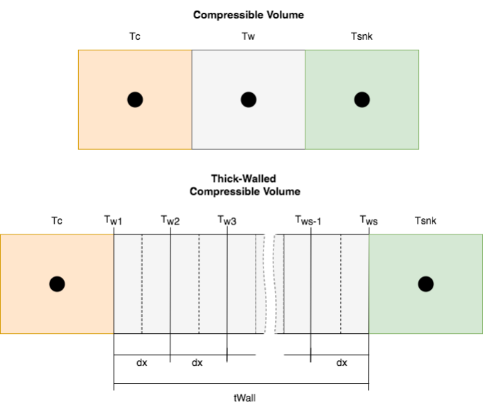
Figure 5.4.4 Geometric representation of a thin-walled (top) and thick-walled (bottom) compressible volume.

A thick-walled compressible volume is divided into s nodes. The first and last node are considered surface nodes, which are half the thickness of the inner nodes. At this time, the material properties within the wall are assumed to be temperature independent and the heat transfer area between each node is constant. The boundary conditions at the inner and outer surface of the wall utilize Newton’s law of cooling. It is assumed that no heat generation occurs within the CV wall. The temperature solution of the CV coolant is consistent between the thin-walled and thick-walled implementation.

5.4.4.1.1. Basic Equations

By combining Eq. (5.3-7) and Eq. (5.4-84), the conservation of energy equation for a thick-walled CV liquid can be written as

(5.4-93) $$T_{4}m_{4} = T_{3}m_{3} + S_3 + S_4T_{4} + \frac{Q}{c_l}\Delta t$$

By replacing the average wall temperature, with the wall surface temperature Eq. (5.4-80) can be written as

(5.4-94) $$Q\Delta t = \Delta t h_wA_w \left( \theta_1\left(T_{w1,3}-T_{3}\right)+\theta_2\left(T_{w1,4}-T_{4}\right)\right)$$

where

$T_{w1,3}$ $T_{w1,4}$ = the compressible volume wall inner surface temperature at the beginning and end of the time step

A similar energy balance can be performed at the inner surface of the compressible volume wall.

(5.4-95) $$(mc)_{w1}T_{w1,4} = (mc)_{w1}T_{w1,3}-Q\Delta t + Q_{w1,w2} \Delta t$$

(5.4-96) $$Q_{w1,w2}\Delta t = \Delta t h_{wi}A_{w} \left( \theta_1\left(T_{w2,3}-T_{w1,3}\right)+\theta_2\left(T_{w2,4}-T_{w1,4}\right)\right)$$

where

(5.4-97) $$h_{wi} = \frac{k}{dx}$$

and

$T_{w2,3}$ $T_{w2,4}$ = the compressible volume wall temperature at node j=2 at the beginning and end of the time step

$k$ = the compressible volume wall thermal conductivity

$s$ = the number of wall nodes

$dx$ = the compressible volume wall node thickness, $\frac{tWall}{s-1}$

$mc_{w1}$ = $mc_{ws}$ = the compressible volume wall surface node heat capacity, $\frac{MCp_{wall}}{2(s-1)}$

The energy balance for the inner wall node, j, will follow a similar pattern

(5.4-98) $$(mc)_{wj}T_{wj,4} = (mc)_{wj}T_{wj,3}-Q_{wj-1,wj}\Delta t + Q_{wj,wj+1} \Delta t$$

(5.4-99) $$Q_{wj-1,wj}\Delta t = \Delta t h_{wi}A_{w} \left( \theta_1\left(T_{wj,3}-T_{wj-1,3}\right)+\theta_2\left(T_{wj,4}-T_{wj-1,4}\right)\right)$$

where

$mc_{wj}$ = the compressible volume wall inner node heat capacity, $\frac{MCp_{wall}}{s-1}$

Finally, the energy balance for the outer surface node can be written

(5.4-100) $$(mc)_{ws}T_{ws,4} = (mc)_{ws}T_{ws,3}-Q_{ws-1,ws}\Delta t + Q_{ws,snk} \Delta t$$

(5.4-101) $$Q_{ws,snk}\Delta t = \Delta t (hA)_{snk} \left( T_{snk} - \left(\theta_1T_{ws,3}+\theta_2T_{ws,4}\right)\right)$$

Eq. (5.4-93) through Eq. (5.4-101) can be rearranged into a tri-diagonal matrix with s+1 rows. Each transient time step, SAS solves for the temperature of the coolant and wall nodes using standard tri-diagonal inversion in subroutine INVRT3. During steady state initialization, an adiabatic boundary condition is applied at the outer surface of the CV wall. As a result, all wall node temperatures can be set to the coolant temperature.

5.4.4.2. CV Input Description

Table 5.4.7 Input in INPMR4 (Block 3) for all CV Models

Variable	Description
NCVP	Number of CVs in the primary loop.
NCVS	Number of CVs in the secondary loop.
ITYPCV	Compressible volume type.
NCCV	Number of sequential CVs with a common cover gas.
ICCVFS	First CV with common cover gas.

Table 5.4.8 Input in INPMR4 (Block 3) for a thick-walled CV

Variable	Description
ThickWallTableID	Table ID for the thick-wall CV table.

Table 5.4.9 Input in PMR4IN (Block 18) for all CV Models

Variable	Range	Description
VOLLGC	>0.0	Total volume, liquid+gas
ALPHAP	/-	Volume pressure expansion coefficient
ALPHAT	/-	Volume temperature expansion coefficient
ZCVL	/-	Reference height for liquid pressure.
AREAIN	>=0.0	Area of liquid-gas interface.
TREFCV	>=0.0	Initial steady-state gas temperature, if present.
BTAPNA	/-	Liquid pressure expansion coefficient
BTATNA	/-	Liquid temperature expansion coefficient
HWALL	/-	Wall-coolant heat transfer coefficient
AWALL	>0.0	CV Wall surface area
CMWALL	>0.0	Heat capacity of the CV wall

Table 5.4.10 Input in the ThickWallTable for the thick-walled CV Model

Column Label	Range	Description
ICV	> 0	ID of CV using a thick-walled approximation.
nNodes	> 2	Number of wall nodes in the thick wall approximation.
kWall	>=0.0	Wall thermal conductivity.
tWall	>=0.0	Wall thickness

Example thick-wall table input:

TABLE <id> ThickWallInput
  ICV   nNodes  kWall   tWall
   3         4  32.4      0.05
   6         3  16.2      0.05
END