5.4.2. Heat Exchangers: Detailed Options

5.4.2.1. Introduction

The Intermediate Heat Exchanger (IHX) and Primary Heat Exchanger (PHX) are characterized by a shell, a primary coolant channel, a tube, and an secondary coolant channel. Under normal conditions the coolant flows down through the primary channel and up through the secondary channel. Flow reversal is included, so that the flow can be either way in either channel. Also, a slant-height parameter is used to permit the flow path through the tube side to be longer than the flow path through the shell side, and a fouling-factor is included to allow for reduced heat transfer in the primary and intermediate flow channels.

The IHX and PHX are modeled as shown in Figure 5.4.2. The shell, primary coolant channel, tube, and secondary coolant channel are divided into between one and 62 vertical sections. The temperatures in the coolants are calculated at the interfaces of the vertical sections, whereas the shell and tube temperatures are calculated at the centers of the vertical sections. In the case of an IHX, the secondary channel is connected at the inlet and outlet to the intermediate loop. In the case of the PHX, the secondary channel is an independent element whose boundary conditions are defined by the user.

The primary flow rate and temperatures at the beginning of the time step as well as the inlet temperatures at the end of the time step are taken from COMMON blocks. Similarly, for an IHX the secondary flow rate and temperatures are taken from COMMON blocks. For a PHX, the secondary flow rate and inlet temperature at the end of the time step are taken from user provided functions. A set of heat transfer equations is set up and solved for the temperatures at the end of the time step. In addition, gravity heads for both the primary and secondary flow channels are calculated using the resulting temperature distributions. The final values are then stored in COMMON blocks.

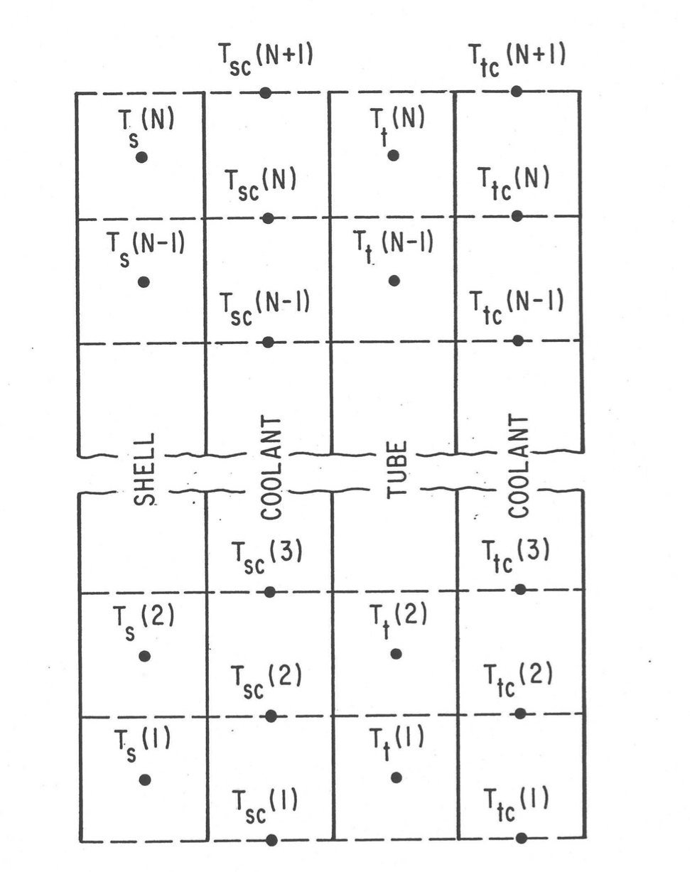
Figure 5.4.2 Intermediate Heat Exchanger Schematic.

5.4.2.2. Basic Equations

In the configuration shown in Figure 5.4.2, a heat balance equation is written for every vertical section of the heat exchanger. Thermal conduction is ignored vertically. The outside surface of the shell can be in thermal contact with a heat sink representing other components or air, as discussed in Section 5.4.6. The heat balance for a vertical section of the shell, which is in thermal contact with the adjacent section of the shell-side liquid, is

(5.4-28) $$\left( \rho c \right)_{\text{SH}}\Delta z P_{\text{s}} d_{\text{SH}} \frac{\partial \text{T}_{\text{SH}}}{\partial \text{t}} = \Delta z P_{\text{s}} H_{\text{s}} \left( {\overline{T}}_{\text{CS}} - T_{\text{SH}} \right) + \Delta z \left( hA \right)_{\text{snk}} \left( T_{\text{snk}} - T_{\text{SH}} \right)$$

with

(5.4-29) $${\overline{T}}_{\text{CS}} = \frac{1}{2} \left\lbrack T_{\text{CS}}\left( j \right) + T_{\text{CS}}\left( j + 1 \right) \right\rbrack$$

(5.4-30) $$\frac{1}{H_{\text{s}}} = \frac{1}{h_{\text{CS}}} + \frac{d_{\text{SH}}}{2k_{\text{SH}}} + \frac{1}{h_{\text{FS}}}$$

(5.4-31) $$h_{\text{CS}} = \frac{{\overline{k}}_{\text{CS}}}{D_{\text{h}}} \left\lbrack C_{1} \left( \frac{D_{\text{h}} \left| \ w_{\text{s}} \right|\ {\overline{c}}_{\text{CS}}}{A_{\text{CS}} {\overline{k}}_{\text{CS}}} \right)^{C_{2}} \left( \frac{ {\overline{c}}_{\text{CS}}{\overline{\mu}}_{\text{CS}}}{{\overline{k}}_{\text{CS}}} \right)^{C_{4}} + C_{3} \right\rbrack$$

where

$\left( \rho c \right)_{\text{SH}}$ = the shell density times specific heat, RCSHHX

$\Delta z$ = the height of the shell section

$P_{\text{S}}$ = the perimeter between the shell and coolant, PERSPX

$d_{\text{SH}}$ = the shell thickness, DSHIHX

$T_{\text{SH}}$ = the temperature of the shell section

$T_{\text{snk}}$ = the temperature of a heat sink outside the shell

$\left( hA \right)_{\text{snk}}$ = the heat transfer coefficient times area per unit height for heat transfer to the sink

$T_{\text{CS}} \left( j \right)$ = the shell-side coolant temperature at the lower end of the vertical section

$T_{\text{CS}} \left( j+1 \right)$ = the shell-side coolant temperature at the upper end of the vertical section

$k_{\text{SH}}$ = the shell thermal conductivity, XKSHHX

$h_{\text{CS}}$ = shell-side coolant heat transfer coefficient

$h_{\text{FS}}$ = user-supplied shell-side coolant channel fouling factor, HFPIHX

${\overline{k}}_{\text{CS}}$ = the primary coolant thermal conductivity at the temperature ${\overline{T}}_{\text{CS}}$

${\overline{c}}_{\text{CS}}$ = the primary coolant specific heat at the temperature ${\overline{T}}_{\text{CS}}$

${\overline{\mu}}_{\text{CS}}$ = the primary coolant viscosity at the temperature ${\overline{T}}_{\text{CS}}$

$\left| \ w_{\text{s}} \right|$ = the absolute value of the shell-side coolant mass flow rate

$D_{\text{h}}$ = the shell-side coolant channel hydraulic diameter, DHELEM

$A_{\text{CS}}$ = the shell-side coolant flow area, AREAEL

$C_1$, $C_2$, $C_3$ , $C_4$ = user-supplied correlation coefficients, C1IHX, C2IHX, C3IHX, C4IHX

The shell density times specific heat and shell thermal conductivity are user-defined constants independent of temperature, whereas the liquid coolant thermal conductivity viscosity and specific heat are evaluated at the average coolant temperature of a vertical section. The fouling factor is a one-parameter effective film coefficient modeling of the heat transfer in a fouled heat exchanger.

The heat balance for a vertical section of the shell-side coolant, which is in thermal contact with the adjacent sections of the shell and of the tube, is

(5.4-32) $$\begin{split} A_{\text{CS}} {\overline{\rho}}_{\text{CS}} {\overline{c}}_{\text{CS}}\Delta z \frac{\partial{\overline{\text{T}}}_{\text{CS}}}{\partial \text{t}} + A_{\text{CS}}\Delta z \frac{w_{\text{S}} {\overline{c}}_{\text{CS}}}{A_{\text{CS}}} \frac{\partial \text{T}_{\text{CS}}}{\partial \text{z}} \\ = \Delta z P_{\text{S}} H_{\text{S}} \left( T_{\text{SH}} - {\overline{T}}_{\text{CS}} \right) + \Delta z P_{\text{ST}} H_{\text{ST}} S \left( T_{\text{TU}} - {\overline{T}}_{\text{CS}} \right)\end{split}$$

with

(5.4-33) $$\frac{1}{H_{\text{ST}}} = \frac{1}{h_{\text{CS}}} + \frac{d_{\text{TU}}}{2k_{\text{TU}}} + \frac{1}{h_{\text{FS}}}$$

where

${\overline{\rho}}_{\text{CS}}$ = the shell-side coolant density evaluated at the temperature ${\overline{T}}_{\text{CS}}$

$w_{\text{S}}$ = the shell-side coolant mass flow rate

$P_{\text{ST}}$ = the perimeter between the shell-side coolant and the tube, PERPTX

$S$ = user-supplied slant height ratio of the tube vertical section, SLANTX

$T_{\text{TU}}$ = the temperature of the tube vertical section

The remaining symbols are the same as defined for the shell.

The slant height ratio enables the user to model the tube-side of the heat exchanger as a coil embedded in the primary coolant. If no slant height is entered in the input, the code sets the slant height to one.

The heat balance for a vertical section of the tube, which is in thermal contact with the adjacent sections of the primary and intermediate coolants is

(5.4-34) $$\begin{split} \left( \rho c \right)_{\text{TU}}\Delta z S \frac{1}{2} \left( P_{\text{ST}} + P_{\text{TT}} \right) d_{\text{TU}} \frac{\partial \text{T}_{\text{TU}}}{\partial \text{t}} \\ = \Delta z S P_{\text{ST}} H_{\text{ST}} \left( {\overline{T}}_{\text{CS}} - T_{\text{TU}} \right) + \Delta z S P_{\text{TT}} H_{\text{TT}} \left( {\overline{T}}_{\text{CT}} - T_{\text{TU}} \right)\end{split}$$

with

(5.4-35) $${\overline{T}}_{\text{CT}} = \frac{1}{2} \left\lbrack T_{\text{CT}} \left( j \right) + T_{\text{CT}} \left( j + 1 \right) \right\rbrack$$

(5.4-36) $$\frac{1}{H_{\text{TT}}} = \frac{1}{h_{\text{CT}}} + \frac{d_{\text{TU}}}{2k_{\text{TU}}} + \frac{1}{h_{\text{FT}}}$$

(5.4-37) $$h_{\text{CT}} = \frac{{\overline{k}}_{\text{CT}}}{D_{\text{h}}} \left\lbrack C_{1} \left( \frac{D_{\text{h}} \left| \ w_{\text{T}} \right|\ {\overline{c}}_{\text{CT}}}{A_{\text{CT}} {\overline{k}}_{\text{CT}}} \right)^{C_{2}} \left( \frac{ {\overline{c}}_{\text{CT}}{\overline{\mu}}_{\text{CT}}}{{\overline{k}}_{\text{CT}}} \right)^{C_{4}} + C_{3} \right\rbrack$$

where

$\left( \rho c \right)_{\text{TU}}$ = the tube density times specific heat, RCTUHX

$\Delta z$ = the height of the tube section

$d_{\text{TU}}$ = the tube thickness, DTUIHX

$T_{\text{CT}} \left( j \right)$ = the tube-side coolant temperature, lower end of the vertical section

$T_{\text{CT}} \left( j+1 \right)$ = the tube-side coolant temperature, upper end of the vertical section

$k_{\text{TU}}$ = the tube thermal conductivity, XKTUHX

$h_{\text{CT}}$ = tube-side coolant heat transfer coefficient

$h_{\text{FT}}$ = user-supplied tube-side coolant channel fouling factor, HFIIHX

${\overline{k}}_{\text{CT}}$ = the tube-side coolant thermal conductivity at the temperature ${\overline{T}}_{\text{CT}}$

${\overline{c}}_{\text{CT}}$ = the tube-side coolant specific heat at the temperature ${\overline{T}}_{\text{CT}}$

${\overline{\mu}}_{\text{CT}}$ = the tube-side coolant viscosity at the temperature ${\overline{T}}_{\text{CT}}$

$\left| w_{\text{T}} \right|$ = the absolute value of the tube-side coolant mass flow rate

$D_{\text{h}}$ = the tube-side coolant channel hydraulic diameter, DHELEM

$A_{\text{CT}}$ = the tube-side coolant flow area, AREAEL

$C_1$, $C_2$, $C_3$, $C_4$ = user-supplied correlation coefficients, C1IHXT, C2IHXT, C3IHXT, C4IHXT

The tube density times specific heat and tube thermal conductivity are user-defined constants independent of temperature, whereas the tube-side coolant thermal conductivity, viscosity and specific heat are evaluated at the average tube-side coolant temperature of the vertical section. The fouling factor is similar to that for the shell side.

The heat balance for a vertical section of the tube-side coolant, which is in thermal contact with only the adjacent section of the tube, is

(5.4-38) $$\begin{split} A_{\text{CT}} {\overline{\rho}}_{\text{CT}} {\overline{c}}_{\text{CT}}\Delta z S \frac{\partial{\overline{\text{T}}}_{\text{CT}}}{\partial \text{t}} + A_{\text{CT}}\Delta z S \frac{w_{\text{T}}{\overline{c}}_{\text{CT}}}{A_{\text{CT}}S}\frac{\partial \text{T}_{\text{CT}}}{\partial \text{z}} \\ = \Delta z S P_{\text{TT}} H_{\text{TT}} \left( T_{\text{TU}} - {\overline{T}}_{\text{CT}} \right)\end{split}$$

where

${\overline{\rho}}_{\text{CT}}$ = tube-side coolant density evaluated at the temperature

$w_{\text{T}}$ = the intermediate coolant mass flow rate

The remaining symbols are the same as already defined in this section.

After the primary and intermediate coolant temperatures have been calculated, as described below, the gravity heads for both coolants are calculated by summing terms like the following for each primary and each intermediate coolant section:

(5.4-39) $$GH = \overline{\rho} g \Delta z$$

where

$GH$ = the gravity head for each coolant section

$\overline{\rho}$ = the average coolant density for a coolant section

$g$ = the acceleration of gravity

$\Delta z$ = the height of the coolant section

5.4.2.3. Finite Difference Equations

If both the shell-side and tube-side coolants did flow through the intermediate heat exchanger in the same direction, the solution would be fairly simple. A set of four simultaneous equations could be solved for each vertical section, and the solutions for all sections could be found by starting at the inlet end and marching the length of the heat exchanger to the exit end. With the flows in opposite directions, however, two approaches are available: iteration or solving a large matrix. Iteration entails guessing one inlet temperature, solving successive sets of 4-by-4 matrices down the length of the IHX, comparing outlet temperatures, and repeating the calculation until outlet temperatures matched. On the other hand, solving a large matrix may involve inverting a 62-by-62 matrix. The iteration method is chosen for the steady-state initialization because that is done only once, and solving the large matrix is chosen for the transient calculation because that is done for each time step.

Eq. (5.4-28), Eq. (5.4-32), Eq. (5.4-34), and Eq. (5.4-38) are converted into difference equations, and the temperature changes during the time step are solved. Time derivatives are replaced by

(5.4-40) $$\begin{aligned} \frac{\partial \text{T}}{\partial \text{t}} = \frac{\Delta T}{\Delta t} && ; && \Delta T = T_{4} - T_{3} \end{aligned}$$

where $T_3$ and $T_4$ are the temperatures at the beginning and at the end of the time interval $\Delta t$. $T_1$ and $T_2$ usually denote the beginning and end of a PRIMAR time step, and any subdivision of that time step is denoted by 3 and 4. Space derivatives are taken in the direction of flow. If the flow is down,

(5.4-41) $$\frac{\partial \text{T}}{\partial \text{z}} = \frac{T\left( j \right) - T\left( j + 1 \right)}{\Delta z}$$

and if the flow is up,

(5.4-42) $$\frac{\partial \text{T}}{\partial \text{z}} = \frac{T\left( j + 1 \right) - T\left( j \right)}{\Delta z}$$

where $T \left( j \right)$ and $T \left( j+1 \right)$ are the temperatures evaluated at the two interfaces of the vertical section of height $\Delta z$. The degree of implicitness is introduced by replacing $T$ with

(5.4-43) $$T = \theta_{1} T_{3} + \theta_{2} T_{4}$$

where $\theta_1 + \theta_2 = 1$, and is described in Section 5.2.4 and in Section 2.8.1 in Chapter 2, and $T_3$ and $T_4$ are the temperatures at the beginning and end of the time interval $\Delta t$.

After making the above substitutions, the equations for the temperature changes during $\Delta t$ for the $j$-th vertical section of the IHX for either direction of flow in either coolant channel can be written as:

For the shell,

(5.4-44) $$a_{1}\left( j \right)\Delta T_{\text{SH}}\left( j \right) + a_{2}\left( j \right)\Delta T_{\text{CS}}\left( j \right) + a_{3}\left( j \right)\Delta T_{\text{CS}}\left( j + 1 \right) = a_{4}\left( j \right)$$

For the shell-side coolant,

(5.4-45) $$\begin{split} e_{1}\left( j \right)\Delta T_{\text{CS}}\left( j \right) + e_{2}\left( j \right)\Delta T_{\text{SH}}\left( j - 1 \right) + e_{3}\left( j \right)\Delta T_{\text{SH}}\left( j \right) \\ + e_{4}\left( j \right)\Delta T_{\text{TU}}\left( j - 1 \right) + e_{5}\left( j \right)\Delta T_{\text{TU}}\left( j \right) + e_{6}\left( j \right)\Delta T_{\text{CS}}\left( j - 1 \right) \\ + e_{7}\left( j \right)\Delta T_{\text{CS}}\left( j + 1 \right) = e_{8}\left( j \right) - e_{9}\left( j \right)\Delta T_{\text{CT}}\left( j - 1 \right) - e_{10}\left( j \right)\Delta T_{\text{CT}}\left( j \right)\end{split}$$

For the tube,

(5.4-46) $$\begin{split} c_{1}\left( j \right)\Delta T_{\text{TU}}\left( j \right) + c_{2}\left( j \right)\Delta T_{\text{CS}}\left( j \right) + c_{3}\left( j \right)\Delta T_{\text{CS}}\left( j + 1 \right) \\ + c_{4}\left( j \right)\Delta T_{\text{CT}}\left( j \right) + c_{5}\left( j \right)\Delta T_{\text{CT}}\left( j + 1 \right) = c_{6}\left( j \right)\end{split}$$

And for the tube-side coolant,

(5.4-47) $$\begin{split} f_{1}\left( j \right)\Delta T_{\text{CT}}\left( j \right) + f_{2}\left( j \right)\Delta T_{\text{TU}}\left( j - 1 \right) + f_{3}\left( j \right)\Delta T_{\text{TU}}\left( j \right) \\ + f_{4}\left( j \right)\Delta T_{\text{CT}}\left( j - 1 \right) + \ f_{5}\left( j \right)\Delta T_{\text{CT}}\left( j + 1 \right) \\ = f_{6}\left( j \right) - f_{7}\left( j \right)\Delta T_{CS}\left( j \right) - f_{8}\left( j \right)\Delta T_{\text{CS}}\left( j + 1 \right)\end{split}$$

The expression for each coefficient in terms of the quantities defined in Section 5.4.2.2 are given in Section 5.16.1.

5.4.2.4. Solution

The solution of Eq. (5.4-44) through Eq. (5.4-47) is carried out by a Gaussian elimination scheme using the zeros present in the matrix. The solution algorithm is given in Section 5.16.2. The solution yields the temperature changes throughout the IHX and PHX during the interval $\Delta t$, and these values are added to the corresponding temperatures at the beginning of the time interval and the results are stored in COMMON blocks.

5.4.2.5. Steady-State Temperatures

The steady-state temperature distributions in the IHX and PHX are obtained from Eq. (5.4-28), Eq. (5.4-32), Eq. (5.4-34), and Eq. (5.4-38) by setting the time-derivative terms to zero and noting that the temperatures at the beginning and at the end of a time interval are the same. In the steady-state solution, an adiabatic boundary condition is used on the outside of the shell. Therefore, the steady-state shell temperatures are the same as the average shell-side coolant temperatures for each vertical section. As a result, only a 3-by-3 matrix equation must be solved for each vertical section in the iterative solution mentioned at the beginning of Section 5.4.2.3. Also only normal coolant flow, down in the primary and up in the secondary, is considered. Finally, once the equilibrium temperature distributions have been determined, the gravity heads for the primary and intermediate flow channels are computed as indicated in Eq. (5.4-39).

The 3-by-3 matrix that must be solved for the $j$-th vertical section is:

(5.4-48) $$\begin{split} \begin{pmatrix} \alpha_{1} + \beta_{1} & - \beta_{1} & 0 \\ - \beta_{1} & \alpha_{2} + \beta_{1} + \beta_{2} & - \beta_{2} \\ 0 & - \beta_{2} & \alpha_{3} + \beta_{2} + \beta_{3} \\ \end{pmatrix} \begin{pmatrix} T_{\text{CS}}\left( j \right) \\ T_{\text{TU}}\left( j \right) \\ T_{\text{CT}}\left( j \right) \\ \end{pmatrix} = \ \begin{pmatrix} D_{1} \\ D_{2} \\ D_{3} \\ \end{pmatrix}\end{split}$$

with

$$\alpha_{1} = \frac{1}{2} \left[ \frac{w_{\text{s}}{\overline{c}}_{\text{CS}}\left( j \right)}{\Delta z\left( j \right) S} - \beta_{1} \right]$$

$$\alpha_{2} = \beta_{1} + \beta_{2}$$

$$\alpha_{3} = - \frac{1}{2} \left[ \frac{w_{\text{T}}{\overline{c}}_{\text{CT}}\left( j \right)}{\Delta z\left( j \right) S} + \beta_{2} \right]$$

$$\beta_{1} = \frac{1}{2} P_{\text{ST}} H_{\text{ST}}\left( j \right)$$

$$\beta_{2} = \frac{1}{2} P_{\text{TT}} H_{\text{TT}}\left( j \right)$$

$$\beta_{3} = 0$$

$$D_{1} = \alpha_{1} T_{\text{CS}} \left( j + 1 \right)$$

$$D_{2} = \beta_{1} T_{\text{CS}} \left( j + 1 \right) + \beta_{2} T_{\text{CT}}\left( j + 1 \right)$$

$$D_{3} = \alpha_{3} T_{\text{CT}} \left( j + 1 \right)$$

where

$w_{\text{S}}$, $w_{\text{T}}$ = the positive steady-state flow rates for the shell and tube sides

The other symbols have the same meanings as in Section 5.4.2.2.

The matrix Eq. (5.4-48) is solved by standard tri-diagonal inversion in subroutine INVRT3.

5.4.2.6. PHX: Boundary Conditions and Coolant Options

The boundary conditions for a PHX are specified using function blocks, defined in Section 2.8.1. The inlet temperature for the secondary coolant should be provided in K within the funcion block iPHXTID. In order to ensure a smooth transition from the steady state calculation to the transient calculation, the inlet temperatures defined in iPHXTID are corrected. The correction factor is defined as the difference between the user provided steady state temperature and the SAS4A/SASSYS‑1 calculated steady state temperature. The flow rate for the secondary coolant should be provided in kg/s within the the function block iPHXWID. The secondary flowrate can be positive (countercurrent) or negative (cocurrent), but flow reversal can not occur during a transient. A cocurrent configuration requires a null transient calculation and is considered an advanced user option.

The coolant type on the secondary side of a PHX can differ from the coolant type on the primary side of the PHX. The secondary coolant is defined using iPHXPRP. The available options for iPHXPRP are the same options available for ICLPRP. If a value is not provided for iPHXPRP, the secondary coolant type is assumed to be the same coolant type as the primary side.

5.4.2.7. HX Input Description

Table 5.4.3 Input in INPMR4 (Block 3) for all HX Models

Variable	Description
NIHX	Number of heat exchangers.
IELIHX	Element number for the primary element in HX IIHX.
ILIHXS	Element number for the secondary element in HX IIHX.
IHXCLC	Model selection parameter for HX IIHX.
ISSIHX	Steady state temperature drop parameter for HX IIHX.

Table 5.4.4 Input in INPMR4 (Block 3) for a PHX Model

Variable	Description
iPHXPRP	Coolant type for secondary element. Optional
iPHXTID	Function ID for secondary element inlet temperature boundary condition.
iPHXWID	Function ID for secondary element flow rate boundary condition.

Table 5.4.5 Input in PMR4IN (Block 18) for all HX Models

Variable	Range	Description
XLENEL	>0.0	Length of the element.
AREAEL	>0.0	Cross-sectional flow area of the liquid element.
DHELEM	>0.0	Hydraulic diameter of liquid element.
ROUGHL	>=0.0	Pipe surface roughness of liquid element
BENDNM	>=0.0	Number of bends in liquid element.
G2PRDR	>=0.0	Initial orifice coefficient of liquid element
WALLMC	>=0.0	Wall heat capacity per unit length of liquid element. Ignored for heat exchanger elements.
WALLH	>=0.0	Wall heat transfer coefficient of liquid element. Ignored for heat exchanger elements.
DTIHX	/-	Optional user specified steady state temperature drop for the primary element within HX.

Table 5.4.6 Input in PMR4IN (Block 18) for the detailed HX Model

Variable	Range	Description
DZSHPX	>=0.0	Fractional axial node heights within HX.
HFPIHX	>=0.0	Fouling heat transfer coefficient for shell side flow within HX.
HFIIHX	>=0.0	Fouling heat transfer coefficient for tube side flow within HX.
SLANTX	>=0.0 <=1.0	Slant-height factor of the tube side flow within HX.
PERSPX	>0.0	Perimeter between shell and shell side coolant within HX.
PERPTX	>0.0	Perimeter between tube and shell side coolant within HX.
PERTIX	>0.0	Perimeter between tube and tube side coolant within HX.
DSHIHX	>0.0	Shell thickness within HX.
DTUIHX	>0.0	Tube thickness within HX.
RCSHHX	>0.0	Volumetric heat capacity of the shell within HX.
RCTUHX	>0.0	Volumetric heat capacity of the tube within HX.
XKSHHX	>0.0	Thermal conductivity of the shell within HX.
XKTUHX	>0.0	Thermal conductivity of the tube within HX.