5.4.1. Pipe Temperatures

The pipe temperature model is a slug flow model with heat transfer to the pipe walls, as indicated in Figure 5.4.1. The coolant in a pipe is divided into a number of moving nodes or slugs. The node boundaries move with the coolant flow. All nodes in a pipe have equal volumes except for the first and last nodes. The inlet node size starts at zero and grows as the flow continues until it reaches the size of the other nodes. At that point a new node is started at the inlet. Similarly, the outlet node shrinks and eventually is removed when its volume reaches zero. The temperature in a coolant node changes due to internal heating (see Direct Element Heating) or heat transfer with the pipe wall, while the temperature in a wall node may change due to internal heating, heat transfer with the coolant, or heat transfer from the outside of the pipe wall. There is one wall node for each coolant node. One radial node is used in the pipe wall. Heat transfer from the outside of the pipe wall is described in Section 5.4.6 on component-to-component heat transfer. Wall nodes do not move, so the wall node in contact with a given coolant node changes periodically as the coolant node boundaries pass wall nodes.

All of the elements in a pipe temperature group are handled at the same time as if they made a single long pipe. The use of equal coolant volumes for each node determines the locations of the wall nodes. If the region represented by a wall node spans the boundary between two elements, then weighted averages are used to obtain the coolant flow area, $A_{\text{c}}$, wall perimeter, $P_{\text{er}}$, wall mass, $M_{\text{w}}$, wall heat capacity, $c_{\text{w}}$, and wall heat-transfer coefficient, $h_{\text{w}}$, for the node. The averaging is done so as to conserve coolant volume and wall mass times heat capacity.

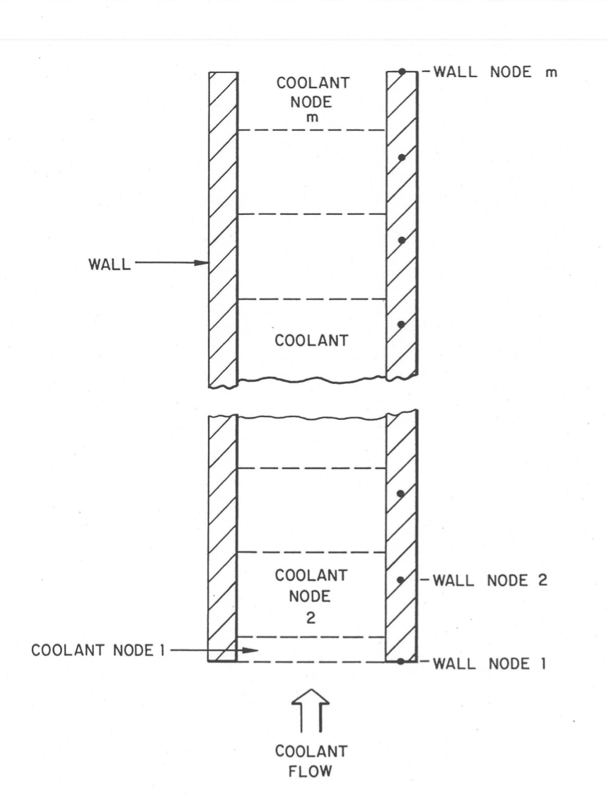
Figure 5.4.1 Pipe Temperature Calculations.

The primary loop time step is divided into sub-intervals for the pipe temperatures calculations. The coolant slug is ejected from the end, a new slug is formed at the inlet, and the node indexes for intermediate slugs are increased by one. In subsequent sub-intervals, the coolant moves exactly one node per sub-interval until the end of the primary loop time step is approached. Usually, the coolant does not move exactly an integral number of nodes in a primary loop step, so in the last sub-interval the coolant usually moves only a fraction of a node.

For any node except the inlet node, the heat-transfer equation used for the coolant is:

(5.4-1) $$\rho_{\text{c}}c_{\text{c}}A_{\text{c}}\frac{\partial \text{T}_{\text{c}}}{\partial \text{t}} = P_{\text{er}} h_{\text{wc}} \left( T_{\text{w}} - T_{\text{c}} \right) + q_{\text{c}}'$$

and that for the wall is

(5.4-2) $$M_{\text{w}}c_{\text{w}}\frac{\partial \text{T}_{\text{w}}}{\partial \text{t}} = P_{\text{er}} h_{\text{wc}} \left( T_{\text{c}} - T_{\text{w}} \right) + \left( \text{hA} \right)_{\text{snk}} \left( T_{\text{snk}} - T_{\text{w}} \right) + q_{\text{w}}'$$

where

$T_{\text{c}}$ = coolant temperature

$T_{\text{w}}$ = wall temperature

$\rho_{\text{c}}$ = coolant density

$c_{\text{c}}$ = coolant specific heat

$h_{\text{wc}}$ = effective heat-transfer coefficient between the wall and the coolant

$M_{\text{w}}$ = wall mass per unit length

$c_{\text{w}}$ = specific heat of the wall

$P_{\text{er}}$ = wall perimeter, $4A/D_h$

$T_{\text{snk}}$ = temperature of a heat sink outside the wall

$\left( hA \right)_{\text{snk}}$ = heat transfer coefficient times area per unit length for heat transfer to air or liquid sodium outside the pipe wall

$q_{\text{c}}'$ = linear heat generation in the coolant

$q_{\text{w}}'$ = linear heat generation in the wall

The effective heat-transfer coefficient $h_{\text{wc}}$ contains a coolant heat-transfer coefficient, $h_{\text{c}}$, in series with a wall heat-transfer coefficient, $h_{\text{w}}$:

(5.4-3) $$\frac{1}{h_{\text{wc}}} = \frac{1}{h_{\text{c}}} + \frac{1}{h_{\text{w}}}$$

or

(5.4-4) $$h_{\text{wc}} = \frac{h_{\text{c}}h_{\text{w}}}{h_{\text{c}} + h_{\text{w}}}$$

The coolant heat-transfer coefficient is calculated as

(5.4-5) $$h_{\text{c}} = \frac{k_{\text{c}}}{D_{\text{h}}} \left\lbrack C_{1}\left( \frac{D_{\text{h}} \left| w \right| c_{\text{c}}}{A_{\text{c}}k_{\text{c}}} \right)^{c_{2}} + C_{3} \right\rbrack$$

$C_1$, $C_2$ and $C_3$ = user-supplied correlation coefficients

$D_{\text{h}}$ = pipe hydraulic diameter

$w$ = coolant flow rate

$k_{\text{c}}$ = thermal conductivity of the coolant

$c_{\text{c}}$ = specific heat of the coolant

The wall heat-transfer coefficient represents heat transfer from the interior of the wall to the surface in contact with the coolant.

Assuming $q_{\text{c}}'$ and $q_{\text{w}}'$ to be constant over a timestep, finite differencing of Eq. (5.4-1) and Eq. (5.4-2) gives

(5.4-6) $$\rho_{\text{c}} c_{\text{c}} A_{\text{c}} \frac{\left( T_{\text{c}6} - T_{\text{c}5} \right)}{\delta t} = \frac{P_{\text{er}}h_{\text{wc}}}{2} \left( T_{\text{w}6} - T_{\text{c}6} + T_{\text{w}5} - T_{\text{c}5} \right) + q_{\text{c}}'$$

and

(5.4-7) $$\begin{split} M_{\text{w}}c_{\text{w}} \frac{\left( T_{\text{w}6} - T_{\text{w}5} \right)}{\delta t} = \frac{P_{\text{er}}h_{\text{wc}}}{2} \left( T_{\text{c}6} - T_{\text{w}6} + T_{\text{c}5} - T_{\text{w}5} \right) \\ + \left( hA \right)_{\text{snk}} \left\lbrack T_{\text{snk}} - \frac{\left( T_{\text{w}6} + T_{\text{w}5} \right)}{2} \right\rbrack + q_{\text{w}}'\end{split}$$

where

$\delta t$ = sub-interval time-step size

$T_{\text{c}5}$ = coolant temperature at beginning of the sub-interval

$T_{\text{c}6}$ = coolant temperature at end of the sub-interval

$T_{\text{w}5}$, $T_{\text{w}6}$ = wall temperatures at the beginning and end of the sub-interval

Simultaneous solution of these equations gives

(5.4-8) $$T_{\text{c}6} = \frac{\left\lbrack d_{2} - d_{1} d_{5} \left( M_{\text{w}} c_{\text{w}} + d_{3} \right) \right\rbrack T_{\text{c}5} + 2M_{\text{w}} c_{\text{w}} d_{1} d_{5} T_{\text{w}5} + 2d_{1} d_{3} d_{5} T_{\text{snk}} + \delta t q_{\text{c}}' + d_1 d_5 \delta t q_{\text{w}}'} {d_{2} + d_{1} d_{5} \left( M_{\text{w}} c_{\text{w}} + d_{3} \right)}$$

and

(5.4-9) $$T_{\text{w}6} = d_{5} \left( M_{\text{w}} c_{\text{w}} - d_{1} - d_{3} \right) T_{\text{w}5} + d_{1} d_{5} \left( T_{\text{c}6} + T_{\text{c}5} \right) + 2d_{3} d_{5} T_{\text{snk}} + d_5 \delta t q_{\text{w}}'$$

where

(5.4-10) $$d_{1} = \frac{\delta t}{2} h_{\text{wc}} P_{\text{er}}$$

(5.4-11) $$d_{2} = \rho_{\text{c}}c_{\text{c}}A_{\text{c}}$$

(5.4-12) $$d_{3} = \frac{\delta t}{2} \left( hA \right)_{\text{snk}}$$

and

(5.4-13) $$d_{5} = \frac{1}{d_{1} + M_{\text{w}} c_{\text{w}} + d_{3}}$$

For the inlet node, the wall temperature calculation is the same as that used for the other nodes, but the coolant temperature calculation is different, since new coolant is being added to the node. The basic equation used for the coolant temperature is

(5.4-14) $$L_{\text{n}} \rho_{\text{c}} c_{\text{c}} A_{\text{c}} \frac{\partial}{\partial \text{t}} \left( f_{\text{r}} T_{\text{c}} \right) = L_{\text{n}} \rho_{\text{c}} c_{\text{c}} A_{\text{c}} {\overline{T}}_{\text{in}} \frac{\partial f_{\text{r}}}{\partial \text{t}} + L_{\text{n}} h_{\text{wc}} P_{\text{er}} f_{\text{r}} \left( T_{\text{w}} - T_{\text{c}} \right) + f_{\text{r}} q_{\text{c}}'$$

where

$L_{\text{n}}$ = length of a full node at the inlet

$f_{\text{r}}$ = fraction of a full node at the inlet

$f_{\text{r}} L_{\text{n}}$ = current length of the inlet node

${\overline{T}}_{\text{in}}$ = pipe inlet temperature

After finite differencing, this equation becomes

(5.4-15) $$\begin{split} \rho_{\text{c}} c_{\text{c}} A_{\text{c}} f_{\text{r}6} T_{\text{c}6} - \rho_{\text{c}} c_{\text{c}} A_{\text{c}} f_{\text{r}5} T_{\text{c}5} = \rho_{\text{c}} c_{\text{c}} A_{\text{c}} {\overline{T}}_{\text{in}} \left( f_{\text{r}6} - f_{\text{r}5} \right) \\ + \frac{\delta t}{2} h_{\text{wc}} P_{\text{er}} \left\lbrack f_{\text{r}5} \left( T_{\text{w}5} - T_{\text{c}5} \right) + f_{\text{r}6} \left( T_{\text{w}6} - T_{\text{c}6} \right) \right\rbrack + f_{\text{r6}} q_{\text{c}}'\end{split}$$

where

$f_{\text{r}5}$ = $f_{\text{r}}$ at beginning of step

$f_{\text{r}6}$ = $f_{\text{r}}$ at end of step.

The simultaneous solution of Eq. (5.4-15) and Eq. (5.4-7) gives

(5.4-16) $$\begin{split} T_{\text{c}6} = \left\{ \left( d_{2} f_{\text{r}5} - d_{1} f_{\text{r}5} + d_{1}^{2} d_{5} f_{\text{r}6} \right) T_{\text{c}5} + d_{1} \left\lbrack f_{\text{r}5} + f_{\text{r}6} d_{5} \left( M_{\text{w}} c_{\text{w}} - d_{1} - d_{3} \right) \right\rbrack T_{\text{w}5} \right. \\ \left. + d_{2} \left( f_{\text{r}6} - f_{\text{r}5} \right) {\overline{T}}_{\text{in}} + 2 f_{\text{r}6} d_{1} d_{3} d_{5} T_{\text{snk}} + f_{\text{r6}} \delta t q_{\text{c}}' + f_{\text{r6}} d_1 d_5 \delta t q_{\text{w}}' \right\} \big/ \\ f_{\text{r}6} \left\lbrack d_{2} + d_{1} d_{5} \left( M_{\text{w}} c_{\text{w}} + d_{3} \right) \right\rbrack\end{split}$$

and Eq. (5.4-9) is again used for the wall temperature.

If flow in the pipe reverses direction, then the temperature calculations are the same, except that the outlet node becomes the inlet node and the inlet node becomes the outlet node.

5.4.1.1. Eulerian Calculations

The slug flow pipe temperature model described above is a LaGrangian treatment that avoids the spurious numerical diffusion that results from typical Eulerian treatments. On the other hand, there are situations in which this treatment requires significantly more computing time than a Eulerian treatment would; and in many of these situations the effects of numerical diffusion would be small, so there is little gain from the time consuming LaGrangian treatment. The Eulerian computation time per subinterval is comparable to the LaGrangian computation time per subinterval, but the LaGrangian time step subinterval size is limited by the restriction that the coolant can not be allowed to move more than one node per subinterval, whereas no such restriction applies in the Eulerian case. Therefore, there is no advantage to a Eulerian treatment if the coolant flow rates are small and the time step sizes are small; but a Eulerian treatment is much faster than a LaGrangian treatment if the coolant flow rate is high and time steps are large enough that the coolant moves many nodes per time step. Therefore, a Eulerian speed-up option has been added to the pipe temperature calculations in the code.

The Eulerian speed-up option can be especially useful in the null transient used for steady-state initialization when component-to-component heat transfer is used. In this case, the temperature time constants are often large, requiring a long null transient to obtain converged temperatures. The temperature solution is numerically stable for large time steps, so one would use a large time step size in the null transient to reduce computing time; but much of the benefit from a large time step size is nullified if a LaGrangian pipe temperature calculation limits the subinterval size to a small value. Also, the numerical diffusion from a Eulerian solution is small or non-existent in a steady-state pipe temperature result, so there is no reason not to use the Eulerian treatment in the null transient.

There are three options for using the Eulerian speed-up. The default option is to always us only the LaGrangian treatment. The second option is to use the Eulerian speed-up in the steady-state null transient but not in the regular transient. The third option is to use the Eulerian speed-up both in the null transient and in the regular transient. In any case, the LaGrangian calculation is used for small time steps in which the coolant will move less than two nodes. If the Eulerian speed-up is being used for a large time step, then first a LaGrangian subinterval is used to move the coolant to the next node boundary. Next, a Eulerian calculation is used to move the coolant the maximum whole number of nodes that will fit within the time step. Finally, a LaGrangian subinterval is used to finish the time step and move the coolant many fraction of a node remaining. The Eulerian part of the calculation is described in Section 5.16.6.

5.4.1.2. Annular Element Temperatures

An annular element is treated the same as a pipe except that an annular element has two walls in contact with the coolant instead of one. The annular element was added to SAS4A/SASSYS‑1 in order to model the coolant flow in an RVACS/RACS system in which a relatively thin annulus of sodium flows between the vessel wall and an inner liner. Significant heat transfer occurs between the sodium in the annulus and both the vessel wall and the inner liner.

For the annular element, the heat transfer equation used for the coolant is

(5.4-17) $$\rho_{\text{c}} c_{\text{c}} A_{\text{c}} \frac{\partial \text{T}_{\text{c}}}{\partial \text{t}} = P_{\text{era}} h_{\text{wca}} \left( T_{\text{wa}} - T_{\text{c}} \right) + P_{\text{erb}} h_{\text{wcb}} \left( T_{\text{wb}} - T_{\text{c}} \right) + q_{\text{c}}'$$

where $P_{\text{era}}$, $h_{\text{wca}}$, and $T_{\text{wa}}$ refer to wall $a$, and $P_{\text{erb}}$, $h_{\text{wcb}}$, and $T_{\text{wb}}$ refer to wall $b$. Eq. (5.4-2) and Eq. (5.4-7) are still applicable to each wall. Finite differencing of Eq. (5.4-17) gives

(5.4-18) $$\begin{split} \rho_{\text{c}} c_{\text{c}} A_{\text{c}} \frac{\left( T_{\text{c}6} - T_{\text{c}5} \right)}{\delta \text{t}} = \frac{P_{\text{era}} h_{\text{wca}}}{2} \left( T_{\text{wa}6} - T_{\text{c}6} + T_{\text{wa}5} - T_{\text{c}5} \right) \\ + \frac{P_{\text{erb}} h_{\text{wcb}}}{2} \left( T_{\text{wb}6} - T_{\text{c}6} + T_{\text{wb}5} - T_{\text{c}5} \right) + q_{\text{c}}'\end{split}$$

Simultaneous solution of the finite difference equations for $T_{\text{c}}$, $T_{\text{wa}}$, and $T_{\text{wb}}$ gives

(5.4-19) $$\begin{split} T_{\text{c}6} = \left\{\left\lbrack d_{2} - d_{1\text{a}} d_{5\text{a}} \left( M_{\text{wa}} c_{\text{wa}} + d_{3\text{a}} \right) - d_{1\text{b}} d_{5\text{b}} \left( M_{\text{wb}} c_{\text{wb}} + d_{3\text{b}} \right) \right\rbrack T_{\text{c}5} \right. \\ \left. + 2d_{1\text{a}} d_{5\text{a}} \left( M_{\text{wa}} c_{\text{wa}} T_{\text{wa}5} + d_{3\text{a}} T_{\text{snka}} + \frac{\delta t}{2} q_{\text{wa}}' \right) \right. \\ \left. + 2d_{1\text{b}} d_{5\text{b}} \left( M_{\text{wb}} c_{\text{wb}} T_{\text{wb}5} + d_{3\text{b}} T_{\text{snkb}} + \frac{\delta t}{2} q_{\text{wb}}' \right) + \delta t q_{\text{c}}' \right\} \\ \big/ \left\lbrack d_{2} + d_{1\text{a}} d_{5\text{a}} \left( M_{\text{wa}} c_{\text{wa}} + d_{3\text{a}} \right) + d_{1\text{b}} d_{5\text{b}} \left( M_{\text{wb}} c_{\text{wb}} + d_{3\text{b}} \right) \right\rbrack\end{split}$$

where $q_{\text{wa}}'$ and $q_{\text{wb}}'$ refer to linear heat sources for walls $a$ and $b$, respectively. The solutions for $T_{\text{wa}}$ and $T_{\text{wb}}$ are the same as Eq. (5.4-9). For the inlet node, simultaneous solution of the finite difference equations gives

(5.4-20) $$\begin{split} T_{\text{c}6} = \left\{ \left\lbrack d_{2} f_{\text{r5}} - d_{1\text{a}} \left( f_{\text{r5}} - f_{\text{r6}} d_{1\text{a}} d_{5\text{a}} \right) - d_{1\text{b}} \left( f_{\text{r5}} - f_{\text{r6}} d_{1\text{b}} d_{5\text{b}} \right) \right\rbrack T_{\text{c}5} \right. \\ \left. + d_{1\text{a}} \left\lbrack f_{\text{r5}} + f_{\text{r6}} d_{5\text{a}} \left( M_{\text{wa}} c_{\text{wa}} - d_{1\text{a}} - d_{3\text{a}} \right) \right\rbrack T_{\text{wa}5} \right. \\ \left. + d_{1\text{b}} \left\lbrack f_{\text{r5}} + f_{\text{r6}} d_{5\text{b}} \left( M_{\text{wb}} c_{\text{wb}} - d_{1\text{b}} - d_{3\text{b}} \right) \right\rbrack T_{\text{wb}5} \right. \\ \left. + d_{2} {\overline{T}}_{\text{in}} \left( f_{\text{r6}} - f_{\text{r5}} \right) + 2f_{\text{r6}} \left\lbrack d_{1\text{a}} d_{3\text{a}} d_{5\text{a}} T_{\text{snka}} + d_{1\text{b}} d_{3\text{b}} d_{5\text{b}} T_{\text{snkb}} \right\rbrack \right. \\ \left. + f_{\text{r6}} \left\lbrack \delta t q_{\text{c}}' + d_{\text{1a}} d_{\text{5a}} \delta t q_{\text{wa}}' + d_{\text{1b}} d_{\text{5b}} \delta t q_{\text{wb}}' \right\rbrack \right\} \\ \big/ f_{\text{r6}} \left\lbrack d_{2} + d_{1\text{a}} d_{5\text{a}} \left( M_{\text{wa}} c_{\text{wa}} + d_{3\text{a}} \right) + d_{1\text{b}} d_{5\text{b}} \left( M_{\text{wb}} c_{\text{wb}} + d_{3\text{b}} \right) \right\rbrack\end{split}$$

5.4.1.3. Direct Element Heating

During operation, heat may be generated and/or removed in a variety of different components. For example, during pump operation, heat may be generated in both the working fluid and in the pump structure itself. This phenomenon may strongly impact system temperatures under certain conditions, and therefore SAS provides users with flexibility when modeling it.

Direct element heating is currently supported in all pipe-like elements. Pipe-like elements include: pipes, pumps, check valves, valves, annular pipes, and annular pumps. Two mechanisms are in place for defining direct element heat, time-dependent functions and built-in pump heat models.

5.4.1.3.1. Time-Dependent Element Heating

Time-dependent functions for direct fluid and direct structure heat can be defined using CoolHeatTableID and WallHeatTableID, respectively.

(5.4-21) $$q_{\text{c}}' = \frac{f_{\text{c,k}}(t)}{L_{\text{k}}}$$

where

$f_{\text{c,k}}$ = user-defined, time-dependent function for element $k$ coolant (W).

$L_{\text{k}}$ = length of element $k$

and

(5.4-22) $$q_{\text{w}}' = \frac{f_{\text{w,k}}(t)}{L_{\text{k}}}$$

where

$f_{\text{w,k}}$ = user-defined, time-dependent function for element $k$ wall (W).

A description of the CoolantHeat Table and the WallHeat Table, identified in CoolHeatTableID and WallHeatTableID, as well as example tables are presented below.

Table 5.4.1 Input in a Direct Coolant Heat Table

Column Label	Description	Range
iEll	Element ID.	1 $\leq$ iEll $\leq$ NELEMT
fID	ID of function defining direct coolant heat for element iELL. The output of this function should be in Watts.

Table 5.4.2 Input in a Direct Wall Heat Table

Column Label	Description	Range
iEll	Element ID. If iEll is greater than 1000, the second wall of iEll-1000 is identifeid.	1 $\leq$ iEll $\leq$ NELEMT
fID	ID of function defining direct wall heat for element iELL. The output of this function should be in Watts.

Example Direct Coolant Heat Table input:

TABLE <id> Coolant
iEll fID
3     1
4   100
END

Example Direct Wall Heat Table input:

TABLE <id> Structure
iEll fID
1003     200
3   100
4   1
END

5.4.1.3.2. Pump Heat

Pump heating is implemented by calculating the contributions to linear heat rates $q_{\text{c}}'$, $q_{\text{w}}'$, $q_{\text{wa}}'$, and $q_{\text{wb}}'$ in the equations above. Currently this treatment is limited only to equivalent circuit pump models, where the scaling factor fH is used to control the fraction of power dissipated in various resistors representing fluid and wall components.

Detailed Equivalent Circuit Model

For reference to the variables cited below, see the governing circuit. Power dissipated by $R_1$ and $R_D$ in each phase is deposited into the element wall while power disspated in $R_J$ is deposited in the fluid. For nodes of element $k$ that corresponds to an equivalent circuit pump, this is expressed as

(5.4-23) $$q_{\text{c}}' = \frac{3 f_H I_3^2 R_J}{L_{\text{k}}}$$

where

$L_{\text{k}}$ = length of element $k$

$I_3$ = current through resistor $R_J$

and

(5.4-24) $$q_{\text{w}}' = \frac{3 f_H \left(I^2 R_1 + I_2^2 R_D \right)}{L_{\text{k}}}$$

If the pump element is annular (see ITYPEL), users can control how much of the wall heat is put into each of $q_{wa}'$ and $q_{wb}'$ as

(5.4-25) $$\begin{split}q_{\text{wa}}' &= f_{OD} q_{\text{w}}' \\ q_{\text{wb}}' &= (1 - f_{OD}) q_{\text{w}}'\end{split}$$

where $f_{OD}$ is fOD.

Simple Equivalent Circuit Model

For reference to the variables cited below, see the governing circuit. Power dissipated by $R_1$ in each phase is deposited into the element wall as

(5.4-26) $$q_{\text{w}}' = \frac{3 f_H I^2 R_1}{L_{\text{k}}}$$

No power is deposited into the coolant in the simple circuit model.

If the pump element is annular (see ITYPEL), users can control how much of the wall heat is put into each of $q_{wa}'$ and $q_{wb}'$ as

(5.4-27) $$\begin{split}q_{\text{wa}}' &= f_{OD} q_{\text{w}}' \\ q_{\text{wb}}' &= (1 - f_{OD}) q_{\text{w}}'\end{split}$$

where $f_{OD}$ is fOD.