12.2. Liquid Slug Flow Rates

The mass flow rate in each of the individual slugs pictured in Figure 12.1.1 is computed from the momentum equation similarly to the calculation of the prevoiding mass flow rate described in Chapter 3. Because of this similarity, the discussion here will be brief and will emphasize the additions that must be made to the model of Chapter 3 to accommodate the fact that there are several separate liquid slugs in the channel rather than one slug which fills the channel as in the prevoiding case. In particular, the model must now be able to handle the fact that the liquid slugs are continually changing length and must account properly for the effect of the bubble vapor pressures in driving the liquid slug flow rates.

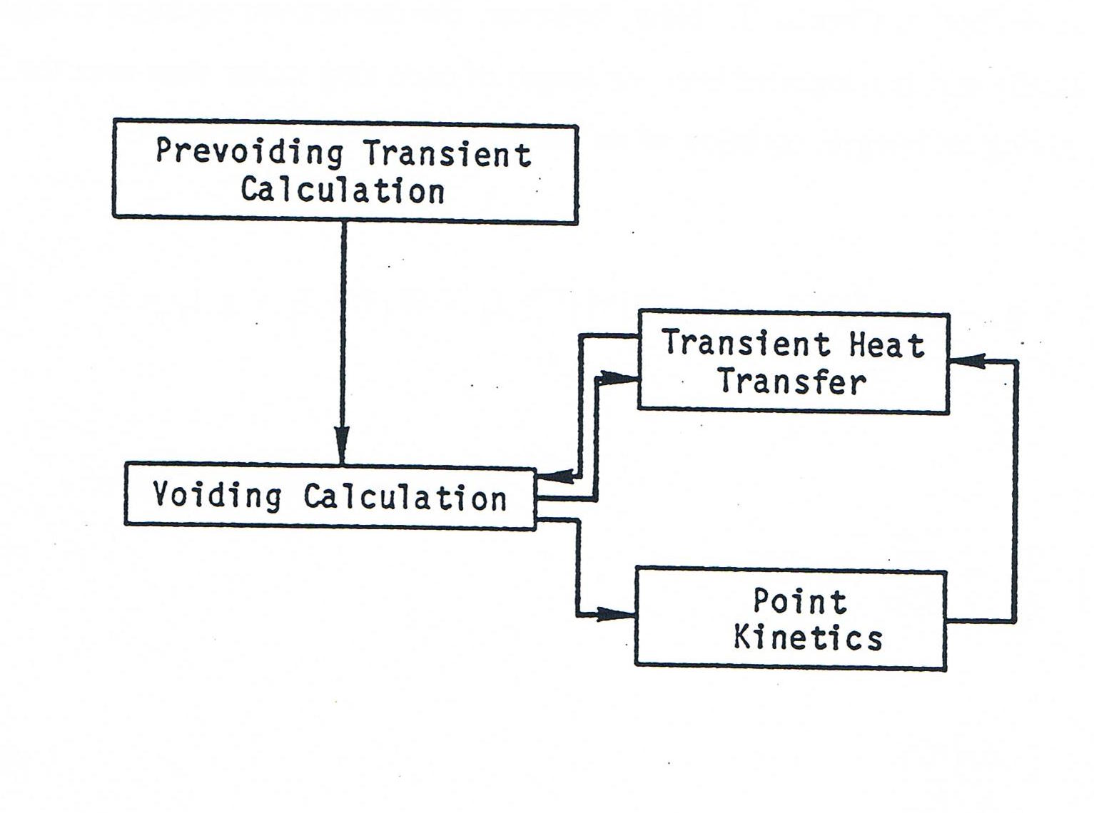
Figure 12.2.1 Schematic Drawing of the Relationship of the Voiding Model to Other SASSYS-1 Models

The foundation of the model is again the liquid momentum equation, Eq. (3.9-1):

(12.2-1) $$\frac{1}{A_{c}}\frac{\partial W}{\partial t} + \frac{\partial p}{\partial z} + \frac{1}{A_{c}}\frac{\partial(Wv)}{\partial z} = - \left( \frac{\partial p}{\partial z} \right)_{fr} - \left( \frac{\partial p}{\partial z} \right)_{K} - \rho_{c}g$$

with the terms as defined in Chapter 3. Now, however, the momentum equation is applied to each slug individually and is integrated over the length of each slug rather than over the length of the channel, giving an integral equation of the form of Eq. (3.9-8):

(12.2-2) $$I_{1}\frac{\partial W}{\partial t} + p_{t} - p_{b} + W^{2}I_{2} + A_{fr}W\left| W \right|^{1 + b_{fr}}I_{3} + W\left| W \right|I_{4} + gI_{5} = 0$$

where

(12.2-3) $$I_{1} = \int_{}^{}{\frac{dz}{A_{c}} =}\sum_{JC = JST}^{JEND}{X_{I1}(JC)}$$

(12.2-4) $$X_{I1}\left( \text{JC} \right) = \frac{\Delta z(JC)}{A_{c}\left( \text{JC} \right)}$$

(12.2-5) $$I_{2} = \sum_{JC = JST}^{JEND}{X_{I2}(JC)}$$

(12.2-6) $$X_{I2}\left( JC \right) = \frac{1}{A_{c}\left( JC \right)^{2}}\lbrack\frac{1}{\rho_{c}(JC + 1)} - \frac{1}{\rho_{c}(JC)}\rbrack$$

(12.2-7) $$I_{3} = \int_{}^{}{\frac{1}{2\rho_{c}A_{c}^{2}D_{h}}\left\lbrack \frac{D_{h}}{\mu A_{c}} \right\rbrack^{b_{fr}}dz = \sum_{JC = JST}^{JEND}{X_{I3}(JC)}}$$

(12.2-8) $$X_{I3}\left( JC \right) = \frac{\Delta z(JC)}{\left\lbrack \rho_{c}\left( JC \right) + \rho_{c}\left( JC + 1 \right) \right\rbrack A_{c}\left( JC \right)^{2}D_{h}(JC)}\left\lbrack \frac{D_{h}\left( \text{JC} \right)}{\overline{\mu}\left( JC \right)A_{c}\left( JC \right)} \right\rbrack^{b_{fr}}$$

(12.2-9) $$I_{4} = \sum_{JC = JST}^{\text{JEND}}{K_{or}(JC)}$$

(12.2-10) $$I_{5} = \int_{}^{}{\rho_{c}dx = \sum_{JC = JST}^{\text{JEND}}{X_{I5}(JC)}}$$

(12.2-11) $$X_{I5}\left( \text{JC} \right) = 0.5\left\lbrack \rho_{c}\left( \text{JC} \right) + \rho_{c}\left( JC + 1 \right) \right\rbrack\Delta z(JC)$$

where

$P_{b} =$ the pressure at the bottom of the slug,

and

$P_{t} =$ the pressure at the top of the slug.

The variable JST is the number of the mesh segment in which the bottom of the liquid slug is located, while JEND is the number of the segment in which the top is contained. The liquid slug configuration in the SASSYS-1 axial mesh is shown in Figure 12.2.1. Note that mesh segments JST and JEND are part liquid and part vapor. Since the integration is over only the liquid portions of these segments, the axial length terms $\Delta z \left( JC \right)$ in the expressions for $X_{I1}$, $X_{I3}$ and $X_{I5}$ must be altered for segments JST and AJEND from being the mesh segment height to being the length of the portion of the segment which is filled with liquid. This is represented by the term $\Delta z'$

(12.2-12) $$\text{If }K > 1,\ \Delta z^{'}\left( JST \right) = z_{c}\left( JST + 1 \right) - z_{i}(L = 1,t,K - 1)$$

(12.2-13) $$\text{If }K = 1,\ \Delta z^{'}\left( JST \right) = \Delta z(JST)$$

(12.2-14) $$\text{If }K \leq K_{vn},\ \Delta z^{'}\left( JEND \right) = z_{i}\left( L = 1,t,k \right) - z_{c}(JEND)$$

(12.2-15) $$\text{If }K > K_{vn},\ \Delta\left( JEND \right) = \Delta z(JEND)$$

The notation $z_i (L,t,K)$ for the interface position is derived from the coding and is to be interpreted as follows. The quantity $L$ takes the value 1 or 2, with $L = 1$ denoting the lower interface of bubble $K$ and $L = 1$ the upper interface. The variable $t$ is simply time, and $K$ is just the bubble number, with the numbering going from 1 for the lowest bubble in the channel to $K_{vn}$ for the highest bubble.

Two other modifications must be made to accommodate the partial segments at the ends of the slug. First, the density $p_c(JST)$ in the expressions for $X_{I2} (JST)$ and $X_{I3} (JST)$ must be replaced by the liquid density at the bubble interface; similarly, $\rho_c (JEND + 1)$ must be replaced by the interface value in $X_{I2} (JEND)$ and $X_{I3} (JEND)$. Second, the terms for JST and JEND in the computation of $I_4$ must be multiplied by the fraction $\Delta z'/\Delta z$.

If JST = 1, the effective inertial term $[\frac{\Delta z_i}{A}]_b$ must be added to $I_1$, and if JEND = MZC, the term $[\frac{\Delta z_i}{A}]_t$ must be included in $I_1$, just as in Chapter 3, Eq. (3.9-9).

In the special case of a small liquid slug entirely contained within one mesh segment, JST = JEND. Then,

(12.2-16) $$\Delta z^{'}\left( \text{JST} \right) = z_{i}\left( L = 1,t,K \right) - z_{i}(L = 2,t,K - 1)$$

and there is only one term in each of the summations for $I_1$ through $I_5$.

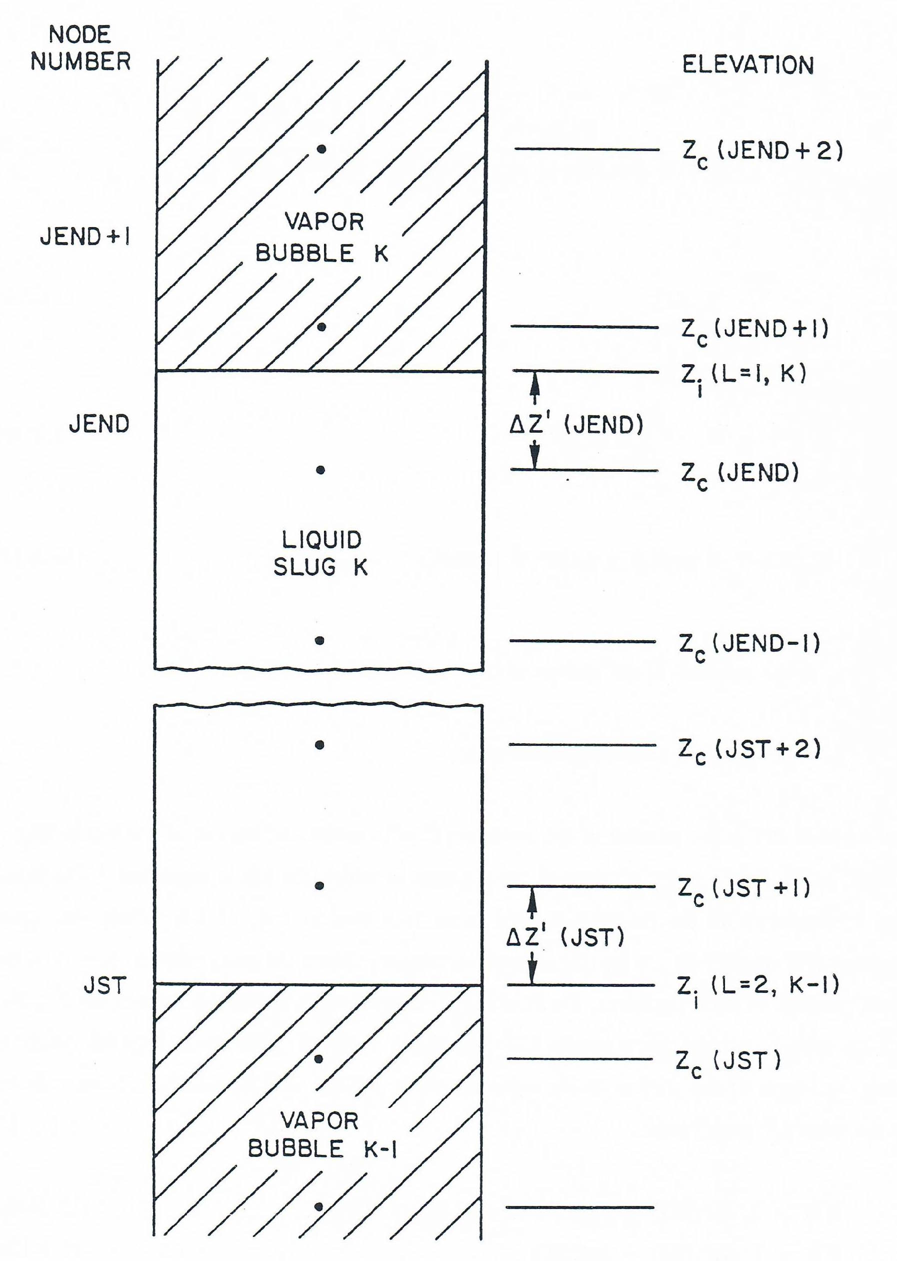
Figure 12.2.2 Placement of a Liquid Slug in the SASSYS-1 Axial Coolant Mesh

Eq. (12.2-2) must now be finite differenced and solved for the liquid mass flow rate in the slug. The advanced time mass flow rate $W$ is forward differenced in time, and functions of $W$ in Eq. (12.2-2) are expressed using first-order Taylor series; see Eq. (3.9-26) through Eq. (3.9-33) for the detailed expressions. However, the differenced form of Eq. (12.2-2) is more complex than the corresponding equation in the prevoiding model, Eq. (3.9-35), because now the coefficients $I_1$ through $I_5$ are functions of time due to motion of the liquid-vapor interfaces, and, therefore, the time level at which these coefficients are evaluated must be specified. To allow flexibility in the level of implicitness of the calculation, the variable explicit/implicit scheme used in Eq. (3.9-26) is applied to the coefficients in Eq. (12.2-2). The differenced equation is then

(12.2-17) $$\begin{split}\left( \theta_{1}I_{1}|_{t} + \theta_{2}I_{1}|_{t + \Delta t} \right)\frac{\Delta W}{\Delta t} + \theta_{1}\left( p_{t_{1}} - p_{b_{1}} \right) + \theta_{2}\left( p_{t_{2}} - p_{b_{2}} \right) \\ + \left( \theta_{1}I_{2}|_{t} + \theta_{2}I_{2}|_{t + \Delta t} \right)\left( W_{1}^{2} + 2\theta_{2}W_{1}\Delta W \right) \\ + A_{fr}\left( \theta_{1}I_{3}|_{t} + \theta_{2}I_{3}|_{t + \Delta t} \right)\big[ W_{1}| W_{1}|^{1 + b_{fr}} \\ + \theta_{2}\left( 2 + b_{fr} \right)\left| W_{1} \right|^{1 + b_{fr}}\Delta W \big] \\ + \left( \theta_{1}I_{4}|_{t} + \theta_{2}I_{4}|_{t + \Delta t} \right)\left( W_{1}|W_{1}| + {2\theta}_{2}|W_{1}|\Delta W \right) \\ + \left( \theta_{1}I_{4}|_{t} + \theta_{2}I_{4}|_{t + \Delta t} \right)g = 0\end{split}$$

The change in the coefficient $I_2$ over a time step is a function only of the change in interface liquid density, which is a very small effect and can be neglected. Therefore, $I_2$ is considered constant over the time step. In addition, the orifice coefficient $I_4$ is also assumed constant over the time step. The advanced time values of the other three coefficients are expressed using forward differencing in time. To illustrate, take the gravity coefficient $I_5$; at time $t$,

(12.2-18) $$I_{5}\left( t \right) = \int_{Z_{\text{JST}}(t)}^{Z_{\text{JEND}}(t)}{\rho_{l}\left( z \right)\text{dz}}$$

and at time $t + \Delta t$,

(12.2-19) $$I_{5}\left( t + \Delta t \right) = \int_{Z_{\text{JST}}(t + \Delta t)}^{Z_{\text{JEND}}(t + \Delta t)}{\rho_{l}\left( z \right)\text{dz}}$$

These two integrals are identical except in segments JST and JEND, where the bubble interface positions are changing with time. Taking the difference gives

(12.2-20) $$I_{5}\left( t + \Delta t \right) - I_{5}\left( t \right) = \int_{Z_{\text{JEND}}\left( t \right)}^{Z_{\text{JEND}}\left( t + \Delta t \right)}{\rho_{l}\left( z \right)\text{dt}} - \int_{Z_{\text{JST}}(t)}^{Z_{\text{JST}}(t + \Delta t)}{\rho_{l}\left( z \right)\text{dz}}$$

The interface position $z_{i}$ can be written as a linear function of the interface velocity $v_{i}$, so that

(12.2-21) $$dz = v_{i}dt$$

Therefore, $I_{5}\left(t + \Delta t \right)$ is

(12.2-22) $$I_{5}\left( t + \Delta t \right) = I_{5}\left( t \right) + \rho_{li}\left( \text{JEND} \right)\int_{t}^{t + \Delta t}{v_{i}\left( L = 1,t^{'},K \right)dt^{'}} - \rho_{li}(JST)\int_{t}^{t + \Delta t}{v_{i}\left( L = 2,t^{'},K - 1 \right)dt'}$$

If the velocity is assumed to vary linearly over the time step, the time integrals in Eq. (12.2-22) become

(12.2-23) $$\begin{align}\begin{aligned}\int_{t}^{t + \Delta t}v_{i}\left( t' \right)dt' &= \overline{v}\Delta t\\&= \left\lbrack v_{i}\left( t \right) + \frac{\Delta v}{2v_{i}\left( t \right)} \right\rbrack\Delta t\\&= v_{i}\left( t \right)\left\lbrack 1 + \frac{\Delta v}{2v_{i}\left( t \right)} \right\rbrack\Delta t\\&= v_{i}\left( t \right)\left\lbrack 1 + \frac{\Delta W}{2W_{1}} \right\rbrack\Delta t\end{aligned}\end{align}$$

where $\Delta v = v_{i} \left(t + \Delta t \right) - v_{i}\left(t\right)$. Therefore, $I_{5}\left(t + \Delta t \right)$ is

(12.2-24) $$\begin{split}I_{5}\left( t + \Delta t \right) = I_{5}\left( t \right) + \rho_{li}\left( \text{JEND} \right)v_{i}\left( L = 1,t,K \right)\left\lbrack 1 + \frac{\Delta W}{2W_{1}} \right\rbrack\Delta t \\ - \rho_{li}\left( \text{JST} \right)v_{i}\left( L = 2,t,K - 1 \right)\left\lbrack 1 + \frac{\Delta W}{2W_{1}} \right\rbrack\Delta t\end{split}$$

This expression is valid for a liquid slug that is bounded at both ends by vapor bubbles. However, slugs that extend out the top of the subassembly do not have a moving upper interface, and so the integral over the upper interface in Eq. (12.2-20) is zero. Similarly, the integral over the lower interface is zero for slugs extending out the bottom of the subassembly. To preserve the ease of using one expression for $I_{5}\left(t + \Delta t \right)$ for all types of liquid slugs, Eq. (12.2-24) is rewritten as

(12.2-25) $$I_{5}\left( t + \Delta t \right) = I_{5}\left( t \right) + \Delta I_{5} + \Delta WI_{5}'$$

where

(12.2-26) $$\Delta I_{5} = \Delta tv_{i}\left( L = 1,t,K \right)\rho_{li}\left( \text{JEND} \right)x_{u} - \Delta tv_{i}\left( L = 2,t,K - 1 \right)\rho_{li}\left( \text{JST} \right)x_{L}$$

(12.2-27) $$I_{5}^{'} = \frac{\Delta I_{5}}{2W_{1}}$$

(12.2-28) $$x_{L} = 1,\ \text{for slug types 2 or 3}$$

(12.2-29) $$x_{L} = 0,\ \text{otherwise}$$

(12.2-30) $$x_{u} = 1,\ \text{for slug types 1 or 2}$$

(12.2-31) $$x_{u} = 0,\ \text{otherwise}$$

Slug type 1 refers to a slug that extends below the subassembly inlet, type 2 to a slug that is bounded top and bottom by bubbles, and type 3 to a slug that extends out the subassembly Table 12.2.1 defines all slug-type numbers used in the code, as well as listing the bubble-type numbers that are part of the coding. Note that the increment $\Delta I_{5}$ represents the change $I_{5}$ if the change in the mass flow rate of the slug is ignored, while the $I_5'$ term accounts for the change due to acceleration of the slug.

The expressions for $I_{1}\left(t + \Delta t \right)$ and $I_{3}\left(t + \Delta t \right)$ are derived in the same way as was Eq. (12.2-25). The resulting equations are

(12.2-32) $$I_{1}\left( t + \Delta t \right) = I_{1}\left( t \right) + \Delta I_{1}$$

where

(12.2-33) $$\Delta I_{1} = \frac{\Delta tv_{i}\left( L = 1,t,K \right)x_{u}}{A_{c}(JEND)} - \frac{\Delta tv_{i}\left( L = 2,t,K - 1 \right)x_{L}}{A_{c}(JST)}$$

(12.2-34) $$I_{3}\left( t + \Delta t \right) = I_{3}\left( t \right) + \Delta I_{3} + \Delta WI_{3}^{'}$$

with

(12.2-35) $$\begin{split}\Delta I_{3} = \frac{\Delta tv_{i}\left( L = 1,t,K \right)x_{u}}{2A_{c}\left( \text{JEND} \right)^{2}\rho_{lt}\left( K \right)D_{h}(JEND)}\left\lbrack \frac{D_{h}\left( \text{JEND} \right)}{A_{c}\left( \text{JEND} \right)\overline{\mu}\left( \text{JEND} \right)} \right\rbrack^{b_{fr}} \\ - \frac{\Delta tv_{i}\left( L = 2,t,K - 1 \right)x_{L}}{2A_{c}\left( \text{JST} \right)^{2}\rho_{lb}\left( K \right)D_{h}\left( \text{JST} \right)}\left\lbrack \frac{D_{h}\left( \text{JST} \right)}{A_{c}(JST)\overline{\mu}\left( \text{JST} \right)} \right\rbrack^{b_{fr}}\end{split}$$

and

(12.2-36) $$I_{3}^{'} = \frac{\Delta I_{3}}{2W_{1}}$$

The effect of slug acceleration is omitted in $I_{1}\left(t + \Delta t \right)$.

Table 12.2.1 Liquid Slug Types and Bubble Types Used in Coolant Dynamics Model

	Bubble Types
	The FORTRAN variable IBUB1 and IBUB2 refer to bubble types.
IBUB	Bubble Type
1	Bubble within the subassembly; uniform vapor pressure bubble.
2	Bubble within the subassembly; pressure gradient model.
3	Bubble extends out the top of the subassembly; uniform vapor pressure bubble.
4	Bubble extends out the top of the subassembly; pressure gradient model.
5	Bubble extends out both the top and bottom of the subassembly.
6	Bubble extends out the bottom of the subassembly.
	Liquid Slug Types
	The FORTRAN variables ILIQ1 and ILIQ2 refer to liquid slug type.
ILIQ	Liquid Slug Type
1	Lower liquid slug, below the lowest bubble.
2	Intermediate liquid slug, with bubbles above and below.
3	Upper liquid slug, above the highest bubble.
4	Liquid slug fills whole subassembly; no voiding.
5	Lower liquid slug below the subassembly inlet, below a type-5 or -6 bubble.
6	Upper liquid slug above the subassembly outlet, above a type-3, -4, or -5 bubble.

Substituting the above expressions for the advanced time coefficients into Eq. (12.2-17) and neglecting second-order terms produces the differenced momentum equation

(12.2-37) $$\begin{split}\left( I_{1} + \theta_{2}\Delta I_{1} \right)\frac{\Delta W}{\Delta t} = \theta_{1}\left( p_{b1} - p_{t1} \right) + \theta_{2}\left( p_{b2} - p_{t2} \right) - I_{2}W_{1}^{2} \\ - 2\theta_{2}\Delta WW_{1}I_{2} - A_{fr}\left( I_{3} + \theta_{2}\Delta I_{3} \right)W_{1}\left| W_{1} \right|^{1 + b_{fr}} \\ - \left( 2 + b_{fr} \right)\theta_{2}A_{fr}I_{3}\left| W_{1} \right|^{1 + b_{fr}}\Delta W \\ - \theta_{2}A_{fr}W_{1}I_{3}^{'}\left| W_{1} \right|^{1 + b_{fr}}\Delta W - I_{4}\left( W_{1}\left| W_{1} \right| + 2\theta_{2}W_{1}\Delta W \right) \\ - g\left( I_{5} + \theta_{2}\Delta I_{5} \right) - gI_{5}^{'}\theta_{2}\Delta W\end{split}$$

which gives

(12.2-38) $$\Delta W = \frac{\Delta t\lbrack AA_{0} + \left( \Delta p_{b} - \Delta p_{t} \right)\theta_{2}\rbrack}{I_{1} + \theta_{2}\Delta I_{1} + \theta_{2}BB_{0}\Delta t}$$

where

(12.2-39) $$AA_{0} = p_{b1} - p_{t1} - I_{2}W_{1}^{2} - A_{fr}\left( I_{3} + \theta_{2}\Delta I_{3} \right)W_{1}\left| W_{1} \right|^{1 + b_{fr}} - I_{4}W_{1}\left| W_{1} \right| - g(I_{5} + \theta_{2}\Delta I_{5})$$

and

(12.2-40) $$BB_{0} = 2W_{1}I_{2} + \left( 2 + b_{fr} \right)A_{fr}I_{3}\left| W_{1} \right|^{1 + b_{fr}} + 2I_{4}\left| W_{1} \right| + A_{fr}\left| W_{1} \right|^{1 + b_{fr}}W_{1}I_{3}^{'} + gI_{5}^{'}$$

Thus the change in flow rate for a liquid slug is related to the changes in vapor pressures in the bubbles above and below the liquid slug, or to the changes in inlet and outlet coolant pressures.