12.6. Vapor Pressure Gradient Model: Large Vapor Bubbles

As mentioned above, whenever a bubble grows to a length greater than a user-specified value (usually 5-50 cm), the vapor bubble calculation is switched from the uniform-vapor-pressure model to a vapor-pressure-gradient model. Saturation conditions are assumed in this model, so the vapor energy equation can be combined with the mass continuity equation. The vapor continuity and momentum equations are solved simultaneously for each node in a bubble using a fully implicit finite differencing scheme.

The equations described in this section are only for the vapor. Any liquid in a bubble region is assumed to be a film on the cladding and structure, and this film is treated separately, as described at the beginning of Section 12.1. The vapor calculation is influenced by the liquid film in only two ways: heat flow through the film provides the vapor source for the vapor calculations; and if a two-phase friction factor multiplier for the friction between the vapor and the film is used, then the film thickness determines the value of this multiplier.

12.6.1. Continuity and Momentum Equations

The vapor continuity equation can be written as

(12.6-1) $$\frac{\partial W}{\partial z} + \frac{\partial\left( \rho_{v}A_{c} \right)}{\partial t} = \frac{Q}{\lambda}A_{C}$$

while the vapor momentum equation is given by

(12.6-2) $$\frac{\partial p}{\partial z} = - \frac{1}{A_{c}}\frac{\partial}{\partial z}\frac{W^{2}}{\rho_{v}A_{c}} - \frac{f_{v}W\left| W \right|}{2\rho_{v}D_{h}A_{c}^{2}} + F_{c} - \frac{1}{A_{c}}\frac{\partial W}{\partial t} - \frac{W\left| W \right|}{2\rho_{v}A_{c}^{2}}\frac{\partial k_{or}}{\partial z}$$

The symbols used in Eq. (12.6-1) and Eq. (12.6-2) are defined as follows:

$W =$ vapor mass flow rate

$z =$ axial height

$\rho_{v} =$ sodium vapor density

$A_{c} =$ coolant flow area

$t =$ time

$Q =$ heat flow rate per unit volume

$\lambda =$ heat of vaporization

$p =$ pressure

$f_{v} =$ friction factor

$D_{h} =$ hydraulic diameter

$F_{c} =$ condensation momentum loss term

$k_{or} =$ orifice pressure drop term

Note that, because the flow area $A_{c}$ is included in the mass and momentum equations as a function of both space and time, the model is able to treat problems involving variable flow areas.

The heat flow rate per unit volume is given by

(12.6-3) $$Q = \gamma\left\lbrack \frac{T_{e} - T}{R_{ec}} + \gamma_{2}\frac{T_{s} - T}{R_{sc}} \right\rbrack$$

where

$\lambda =$ ratio of cladding surface area to coolant volume

$T_{e} =$ cladding temperature

$T_{s} =$ structure temperature

$T =$ vapor temperature

$R_{ec} =$ thermal resistance between the cladding and the vapor

$R_{sc} =$ thermal resistance between the structure and the vapor

$\gamma_{2} =$ ratio of structure surface are to cladding surface area

The thermal resistances $R_{ec}$ and $R_{sc}$ account for the resistance to heat flow of the cladding, liquid film, and vapor and are computed according to the expressions discussed in Section 12.5.1.

The expression for the heat flow rate $Q$ can be rewritten as the sum of the heat flow rate through the cladding, $Q_{e}$, and the heat flow rate through the structure, $Q_{s}$, where

(12.6-4) $$Q_{e} = \gamma\frac{T_{e} - T}{R_{ec}}$$

and

(12.6-5) $$Q_{s} = \gamma\gamma_{2}\frac{T_{s} - T}{R_{sc}}$$

These two quantities are used to compute the condensation momentum loss term $F_{c}$. This term accounts for momentum lost from the system when flowing sodium vapor condenses on cladding or structure that is colder than the vapor. Only a momentum loss term is included, since it is assumed that the system does not gain momentum when vaporization occurs from cladding or structure that is hotter than the sodium film. The condensation momentum loss is simply the product of the rate of mass condensing per unit volume, $\frac{Q}{\lambda}$, times the average velocity, $\frac{W}{2\rho_{v}A_{c}}$. Splitting the condensation momentum loss term into separate contributions from the cladding and structure then gives.

(12.6-6) $$F_{c} = F_{ce} + F_{cs}$$

where

(12.6-7) $$\begin{split}F_{ce} = \begin{cases} 0 & Q_{e} \geq 0, \\ \frac{Q_{e}W}{2\rho_{v}A_{c}\lambda} & Q_{e} < 0 \end{cases}\end{split}$$

and

(12.6-8) $$\begin{split}F_{cs} = \begin{cases} 0 & Q_{s} \geq 0, \\ \frac{Q_{s}W}{2\rho_{v}A_{c}\lambda} & Q_{s} < 0 \end{cases}\end{split}$$

These definitions reflect the assumption that momentum is lost when condensation of vapor occurs ($Q_{e}$, $Q_{s}$ negative) but that no momentum change occurs when liquid is vaporized ($Q_{e}$, $Q_{s}$ positive).

The friction factor, $f_{v}$ is expressed as

(12.6-9) $$f_{v} = A_{fr}\left( \frac{D_{h}\left| W \right|}{\mu A_{c}} \right)^{b_{fr}}f_{tp}$$

where $\mu$ is the vapor viscosity and $A_{fr}$ and $b_{fr}$ are input constants. The quantity in parentheses, $D_{h}|W|/\left( \mu A_{c} \right)$, is just the Reynolds number of the sodium vapor. The two-phase friction factor multiplier, $f_{tp}$, is based on a correlation by Wallis [12-10]:

(12.6-10) $$f_{tp} = 1 + 300 f_{2\phi}(w_{fe} + \gamma_{2}w_{fs})/\lbrack\left( 1 + \gamma_{2} \right)D_{h}\rbrack$$

where $f_{2\phi}$ is set to 1.0 when the two-phase multiplier is used and is set to 0 by the user if a smooth tube friction factor is described.

Two approximations are made to Eq. (12.6-1) and Eq. (12.6-2) before finite differencing. First, in the continuity equation, the term

(12.6-11) $$\frac{\partial(\rho_{v}A_{c})}{\partial t} = \rho_{v}\frac{\partial A_{c}}{\partial t} + A_{c}\frac{\partial\rho_{v}}{\partial t}$$

is taken to be

(12.6-12) $$\frac{\partial(\rho_{v}A_{c})}{\partial t} = A_{c}\frac{\partial\rho_{v}}{\partial t}$$

So that $A_{c}$ is assumed constant in time (but not space) over the time step for purposes fo solving the mass and momentum equations for the vapor pressures and mass flow rates. This assumption is also made with the variables $D_{h}$, $\gamma$, and $\gamma_{2}$. This simplification is a reasonable one, since one of these four quantities changes rapidly with time. Second, in the momentum equations, the momentum convection term can be expanded as

(12.6-13) $$\frac{\partial}{\partial z}\left( \frac{W^{2}}{\rho_{v}A_{c}} \right) = \frac{1}{A_{c}}\frac{\partial}{\partial z}\left( \frac{W^{2}}{\rho_{v}} \right) + \frac{W^{2}}{\rho_{v}}\frac{\partial}{\partial z}\left( \frac{1}{A_{c}} \right)$$

Any changes in area over a spatial node are incorporated into the orifice term, and so $\frac{W^{2}}{\rho_{v}}\frac{\partial}{\partial z}(\frac{1}{A_{c}})$ is included in the $\frac{\partial k_{or}}{\partial z}$ term. Therefore,

(12.6-14) $$\frac{\partial}{\partial z}\left( \frac{W^{2}}{\rho_{v}A_{c}} \right) = \frac{1}{A_{c}}\frac{\partial}{\partial z}\left( \frac{W^{2}}{\rho_{v}} \right)$$

so $A_{c}$ appears piecewise constant in space. This is also true for $D_{h}$, $\gamma$, and $\gamma_{2}$.

Therefore, the continuity and momentum equations to be differenced are

(12.6-15) $$\frac{\partial W}{\partial z} + A_{c}\frac{\partial\rho_{v}}{\partial t} = \frac{Q}{\lambda}A_{c}$$

and

(12.6-16) $$\frac{\partial p}{\partial z} = - \frac{1}{A_{c}^{2}}\frac{\partial}{\partial z}\left( \frac{W^{2}}{\rho_{v}} \right) - A_{fr}\frac{W\left| W \right|^{1 + b_{fr}}}{2\rho_{v}D_{h}^{1 - b_{fr}}A_{c}^{2 + b_{fr}}} + F_{c} - \frac{1}{A_{c}}\frac{\partial W}{\partial t} - \frac{W\left| W \right|}{2\rho_{v}A_{c}^{2}}\frac{\partial k_{or}}{\partial z}$$

12.6.2. Finite Differencing

The mass and momentum equations must now be reduced to algebraic equations that can be coded into SASSYS-1. This is accomplished in three steps: (1) the equations are discretized using finite differences, (2) the advanced time terms are linearized, and (3) saturation conditions are imposed to limit the independent variables to the change in mass flow rate and the change in pressure. The details of these three steps are presented below. The result is the set of algebraic equations Eq. (12.6-45), Eq. (12.6-79), Eq. (12.6-87) (discretized form of the continuity equation at an interior node, lower interface, and upper interface of a bubble, respectively), Eq. (12.6-132), Eq. (12.6-147), and Eq. (12.6-153) (discretized form of the momentum equation in the interior, the lower interface, and the upper interface). These equations are then solved according to the procedure discussed in Section 12.6.3.

As indicated in Figure 12.6.1, some of the variables in the mass and momentum equations are calculated at node boundaries, whereas others are calculated at node mid-points. In general, midpoint quantities are used as if they were constant over the node. The quantities defined at node boundaries are $z$, $T$, $p$, $W$, $\rho_{v}$, $\mu$, and the velocity $V$. At liquid-vapor interfaces, these quantities are defined at the interface, and the vapor velocity is set to the value of the interface velocity.

Midpoint quantities include $T_{e}$, $T_{s}$, $R_{ec}$, $A_{c}$, $D_{h}$, $\gamma$, $\gamma_{2}$, $k_{or}$, $\gamma$, $Q$, $F_{e}$, and the spatially averaged coolant temperature $\overline{T}$. With all variables, a subscript 1 indicates that the variable is evaluated at the beginning of the time step; a subscript 2 means the variable is taken to be at the end of the time step.

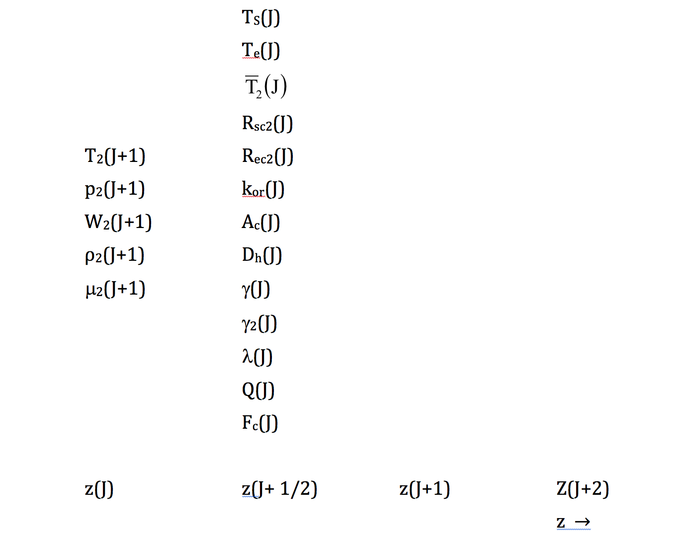
Figure 12.6.1 SASSYS-1 Voiding Model Axial Coolant Mesh Variable Placement

12.6.2.1. Finite Differencing of the Continuity Equation for a Mesh Segment Contained Entirely in One Bubble

This section gives a detailed explanation of how the continuity equation is expressed in finite difference form. The extra factors required to model bubble-liquid interfaces correctly are not included here; they will be discussed in Section 12.6.2.2. Therefore, the equations to be developed in this section apply as they stand only to axial mesh segments which are entirely contained within the bubble.

12.6.2.1.1. Differencing of the Continuity Equation

The terms making up the continuity equation are differenced as follows:

(12.6-17) $$\left. \frac{\partial W}{\partial z} \right|_{J + 1/2} = \frac{W_{2}(J + 1) - W_{2}(J)}{z(J + 1) - z(J)}$$

and

(12.6-18) $$A_{c}\left. \frac{\partial\rho_{v}}{\partial t} \right|_{J + 1/2} = A_{c}(J)\frac{\rho_{2}(J) - \rho_{1}(J) + \rho_{2}(J + 1) - \rho_{1}(J + 1)}{2\Delta t}$$

These differencing schemes are illustrated in Figure 12.6.2. Also,

(12.6-19) $$\begin{align}\begin{aligned}Q_{2}(J) &= \gamma(J)\left\lbrack \frac{T_{e_2}(J) - {\overline{T}}_{2}(J)}{R_{{ec}_2}} + \gamma_{2}(J)\frac{T_{s_{2}}(J) - {\overline{T}}_{2}(J)}{R_{sc_{2}}(J)} \right\rbrack\\&= Q_{e_{2}}(J) + Q_{s_{2}}(J)\end{aligned}\end{align}$$

Therefore, the differenced continuity equation becomes

(12.6-20) $$\begin{split}\frac{W_{2}(J + 1) - W_{2}(J)}{z(J + 1) - z(J)} + A_{c}(J)\frac{\rho_{2}(J) - \rho_{1}(J) + \rho_{2}(J + 1) - \rho_{1}(J + 1)}{2\Delta t} \\ = A_{c}(J)\frac{Q_{2}(J)}{\lambda_{2}(J)}\end{split}$$

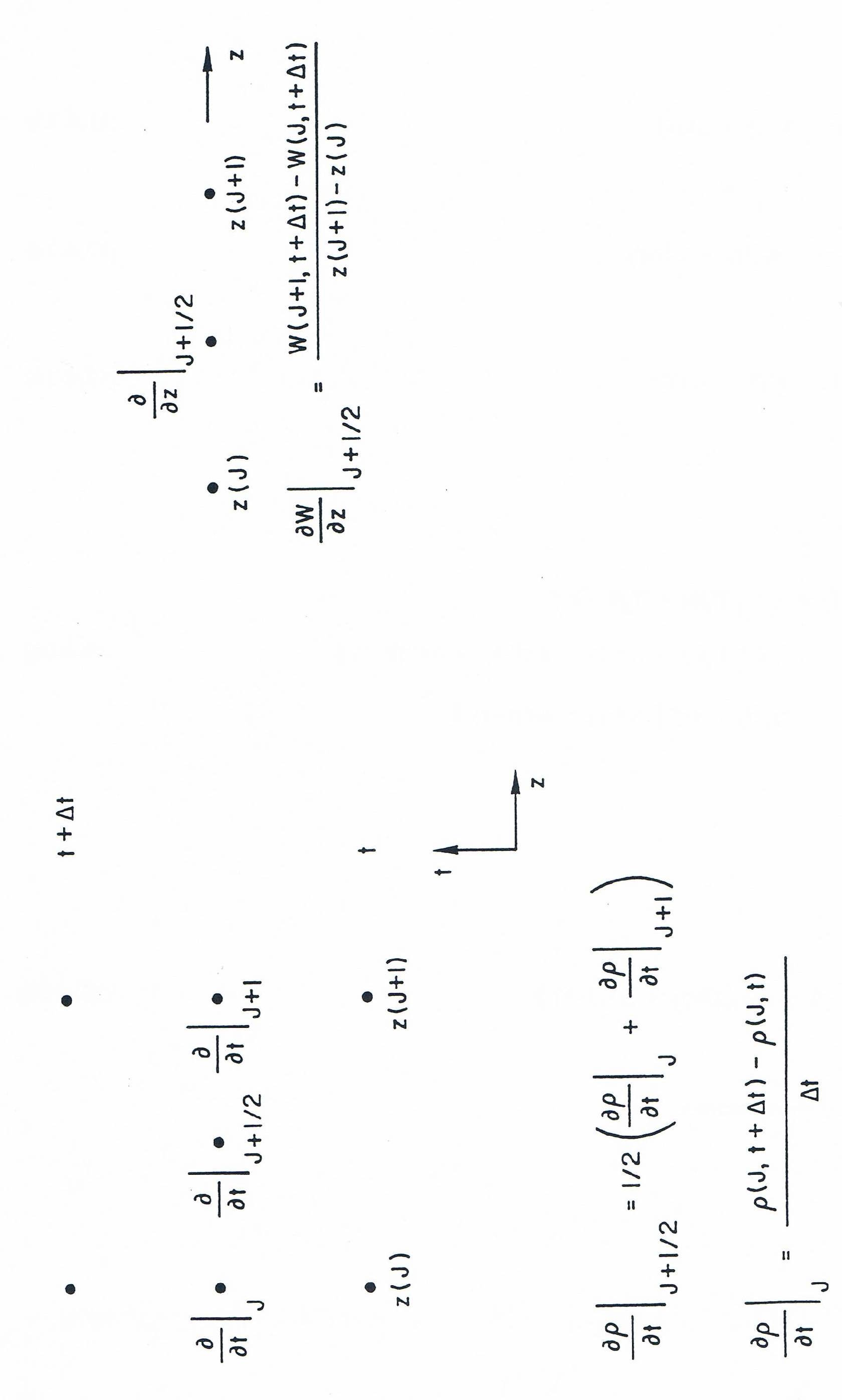
Figure 12.6.2 Evaluation of Derivatives at an Interior Node in the SASSYS-1 Voiding Model

12.6.2.1.2. Linearization of Advanced Time Terms

Eq. (12.6-20) can be linearized by expressing the advanced time terms in the form

(12.6-21) $$x_{2}(J) = x_{1}(J) + \Delta x(J)$$

where x is any quantity. This produces

(12.6-22) $$\rho_{2}(J) = \rho_{1}(J) + \Delta\rho(J)$$

(12.6-23) $$\lambda_{2}(J) = \lambda_{1}(J) + \Delta\lambda(J)$$

(12.6-24) $$W_{2}(J) = W_{1}(J) + \Delta W(J)$$

(12.6-25) $$T_{2}(J) = T_{1}(J) + \Delta T(J)$$

Since

(12.6-26) $$\begin{align}\begin{aligned}\overline{T}_{2}(J) &= \frac{1}{2}\left( T_{2}(J) + T_{2}(J + 1) \right)\\&= \frac{1}{2}\left( T_{1}(J) + \Delta T(J) + T_{1}(J + 1) + \Delta T(J + 1) \right)\\&= \overline{T}_{1}(J) + \frac{1}{2}(\Delta T(J) + \Delta T(J + 1))\end{aligned}\end{align}$$

then

(12.6-27) $$\Delta\overline{T}(J) = \frac{1}{2}\left( \Delta T(J) + \Delta T(J + 1) \right)$$

The heat flux then becomes

(12.6-28) $$\begin{split}Q_{2}(J) = \gamma(J)\left[\frac{T_{e_{2}}(J) - {\overline{T}}_{1}(J) - \Delta\overline{T}(J)}{R_{ec_{2}}(J)} + \gamma_{2}(J)\frac{T_{s_{2}}(J) - {\overline{T}}_{1}(J) - \Delta\overline{T}(J)}{R_{{sc}_2}(J)}\right] \\ = \gamma(J)\Bigg[ \frac{T_{e_{2}}(J) - {\overline{T}}_{1}(J)}{R_{ec_{2}}(J)} + \gamma_{2}(J)\frac{T_{s_{2}}(J) - {\overline{T}}_{1}(J)}{R_{{sc}_2}(J)} \\ - \frac{\left( \Delta T(J) + \Delta T(J + 1) \right)}{2}\left\lbrack \frac{1}{R_{ec_{2}}(J)} + \frac{\gamma_{2}(J)}{R_{sc_{2}}(J)} \right\rbrack \Bigg]\end{split}$$

The heat flux expression can be written in a more compact form by defining the variable $Q_{o}(J)$

(12.6-29) $$Q_{0}(J) = \gamma(J)\left\lbrack \frac{T_{e_{2}}(J) - \overline{T}(J)}{R_{ec_{2}}(J)} + \gamma_{2}(J)\frac{T_{s_{2}}(J) - {\overline{T}}_{1}(J)}{R_{sc_{2}}(J)} \right\rbrack$$

The derivative with respect to vapor temperature of $Q_{o}$ is then

(12.6-30) $$\frac{dQ_{0}}{dT_{J}} = - \gamma(J)\left\lbrack \frac{1}{R_{ec_{2}}(J)} + \frac{\gamma_{2}(J)}{R_{sc_{2}}(J)} \right\rbrack$$

These can be substituted into the above equation for $Q_{2}(J)$ to give

(12.6-31) $$Q_{2}(J) = Q_{0}(J) + \frac{1}{2}\frac{dQ_{0}}{dT_{J}}\left( \Delta T(J) + \Delta T(J + 1) \right)$$

Substituting Eq. (12.6-22) through Eq. (12.6-25) and Eq. (12.6-31) for the advanced time terms in the differenced continuity equation, Eq. (12.6-20) gives

(12.6-32) $$\begin{split}\frac{W_{1}(J + 1) - W_{1}(J) + \Delta W(J + 1) - \Delta W(J)}{z(J + 1) - z(J)} + A_{c}(J)\frac{\Delta\rho(J) + \Delta\rho(J + 1)}{2\Delta t} \\ = \frac{A_{c}(J)}{\lambda_{1}(J) + \Delta\lambda(J)}\left( Q_{0}(J) + \frac{1}{2}\frac{dQ_{0}}{dT_{J}}\left( \Delta T(J) + \Delta T(J + 1) \right) \right)\end{split}$$

If $\Delta \lambda (J) \ll \lambda_{1}(J)$,

(12.6-33) $$\frac{1}{\lambda_{1}(J) + \Delta\lambda(J)} \approx \frac{1}{\lambda_{1}(J)}\left[1 - \frac{\Delta\lambda(J)}{\lambda_{1}(J)}\right]$$

which changes Eq. (12.6-32) to

(12.6-34) $$\begin{split}\frac{W_{1}(J + 1) - W_{1}(J) + \Delta W(J + 1) - \Delta W(J)}{z(J + 1) - z(J)} + A_{c}(J)\frac{\Delta\rho(J) + \Delta\rho(J + 1)}{2\Delta t} \\ = A_{c}(J)\frac{Q_{0}(J)}{\lambda_{1}(J)}\left( 1 + \frac{\Delta T(J) + \Delta T(J + 1)}{2Q_{0}(J)}\frac{dQ_{0}}{dT_{J}} \right)\left( 1 - \frac{\Delta\lambda(J)}{\lambda_{1}(J)} \right)\end{split}$$

Eliminating second-order terms gives the linearized differenced continuity equation

(12.6-35) $$\begin{split}\frac{W_{1}(J + 1) - W_{1}(J) + \Delta W(J + 1) - \Delta W(J)}{z(J + 1) - z(J)} + A_{c}(J)\frac{\Delta\rho(J) + \Delta\rho(J + 1)}{2\Delta t} \\ = A_{c}(J)\frac{Q_{0}(J)}{\lambda_{1}(J)}\left(1 + \frac{\Delta t(J) + \Delta T(J + 1)}{2Q_{0}(J)}\frac{dQ_{0}}{dT_{J}} - \frac{\Delta\lambda(J)}{\lambda_{1}(J)}\right)\end{split}$$

12.6.2.1.3. Utilization of Saturation Conditions to Limit the Independent Variables to $\Delta W$ and $\Delta p$

Since saturation conditions are assumed, $\rho$, $T$, and $\lambda$ are all functions of $p$ only. Therefore, the difference terms can be expressed in terms of $\Delta p$ as follows:

(12.6-36) $$\Delta T(J) = \Delta p(J)\frac{dT}{dp_{J}}$$

(12.6-37) $$\Delta\rho(J) = \Delta p(J)\frac{d\rho}{dp_{J}}$$

(12.6-38) $$\Delta\lambda(J) = \frac{1}{2}\left( \Delta p(J) + \Delta p(J + 1) \right)\frac{d \lambda}{dp_{J}}$$

with $\Delta p (J) = p_{2} (J) - p_{1} (J)$. All derivatives are evaluated at the start of the time step. When Eq. (12.6-36) through Eq. (12.6-38). are inserted into Eq. (12.6-35) the result is a differenced continuity equation which is linear in $\Delta W$ and $\Delta p$:

(12.6-39) $$\begin{split}\frac{W_{1}(J + 1) - W_{1}(J) + \Delta W(J + 1) - \Delta W(J)}{z(J + 1) - z(J)} + A_{c}(J)\frac{1}{2\Delta t}\left( \Delta p(J)\frac{d\rho}{dp_{J}} + \Delta p(J + 1)\frac{d\rho}{dp}(J + 1) \right) \\ = A_{c}(J)\frac{Q_{0}(J)}{\lambda_{1}(J)}\Bigg[ 1 + \left( \Delta p(J)\frac{dT}{dp_{J}} + \Delta p(J + 1)\frac{dT}{dp_{J + 1}} \right)\frac{1}{2Q_{0}(J)}\frac{dQ_{0}}{dT_{J}} \\ - \left( \Delta p(J) + \Delta p(J + 1) \right)\frac{1}{2\lambda_{1}(J)}\frac{d\lambda}{dp_{J}} \Bigg]\end{split}$$

Multiply through by $\left(z(J + 1) - z(J)\right) \Delta t$ and define the coefficients

(12.6-40) $$c_{1,j} = \left( z(J + 1) - z(J) \right)A_{c}(J)\left\lbrack\frac{1}{2}\frac{d\rho}{dp_{J}} - \frac{\Delta t}{2\lambda_{1}(J)}\frac{dT}{dp_{J}}\frac{dQ_{0}}{dT_{J}} + \frac{Q_{0}(J)\Delta t}{2\lambda_{1}^{2}(J)}\frac{d\lambda}{dp_{J}}\right\rbrack$$

(12.6-41) $$c_{2,j} = - \Delta t$$

(12.6-42) $$c_{3,j} = \left( z(J + 1) - z(J) \right)A_{c}(J)\left\lbrack \frac{1}{2}\frac{d\rho}{dp_{J + 1}} - \frac{\Delta t}{2\lambda_{1}(J)}\frac{dT}{dp_{J + 1}}\frac{dQ_{0}}{dT_{J}} + \frac{Q_{0}(J)\Delta t}{2\lambda_{1}^{2}(J)}\frac{d\lambda}{dp_{J}} \right\rbrack$$

(12.6-43) $$c_{4,J} = \Delta t$$

Also, define the source term

(12.6-44) $$h_{J} = W_{1}(J) - W_{1}(J + 1) + \left( z(J + 1) - z(J) \right)A_{c}(J)\frac{Q_{0}(J)}{\lambda_{1}(J)}\Delta t$$

Then the differenced mass equation becomes

(12.6-45) $$c_{1,J}\Delta p(J) + c_{2,J}\Delta W(J) + c_{3,J}\Delta p(J + 1) + c_{4,J}\Delta W(J + 1) = h_{j}$$

12.6.2.2. Finite Differencing of the Continuity Equation for a Mesh Segment Which Contains a Bubble Interface

12.6.2.2.1. Adjustment of the Form of the Continuity Equation to Account for Interface Motion

The representation of the partial derivative with respect to time is not as straightforward at an interface as it is at an interior node. Referring to Figure 12.6.3, in which node boundary $J$ is the interface, the partial derivative of the density $\rho$ is still calculated as

(12.6-46) $$\left. \frac{\partial\rho}{\partial t} \right|_{J + 1/2} = \frac{1}{2}\left\lbrack \left. \frac{\partial\rho}{\partial t} \right|_{J} + \left. \frac{\partial\rho}{\partial t} \right|_{J + 1} \right\rbrack$$

The partial derivatives at $J$ and $J + 1$ are computed just as they are for an interior node; in particular,

(12.6-47) $$\left. \frac{\partial\rho}{\partial t} \right|_{J} = \frac{\rho\left( z\left( J,t \right),t + \Delta t \right) - \rho\left(z\left( J,t \right),t\right)}{\Delta t}$$

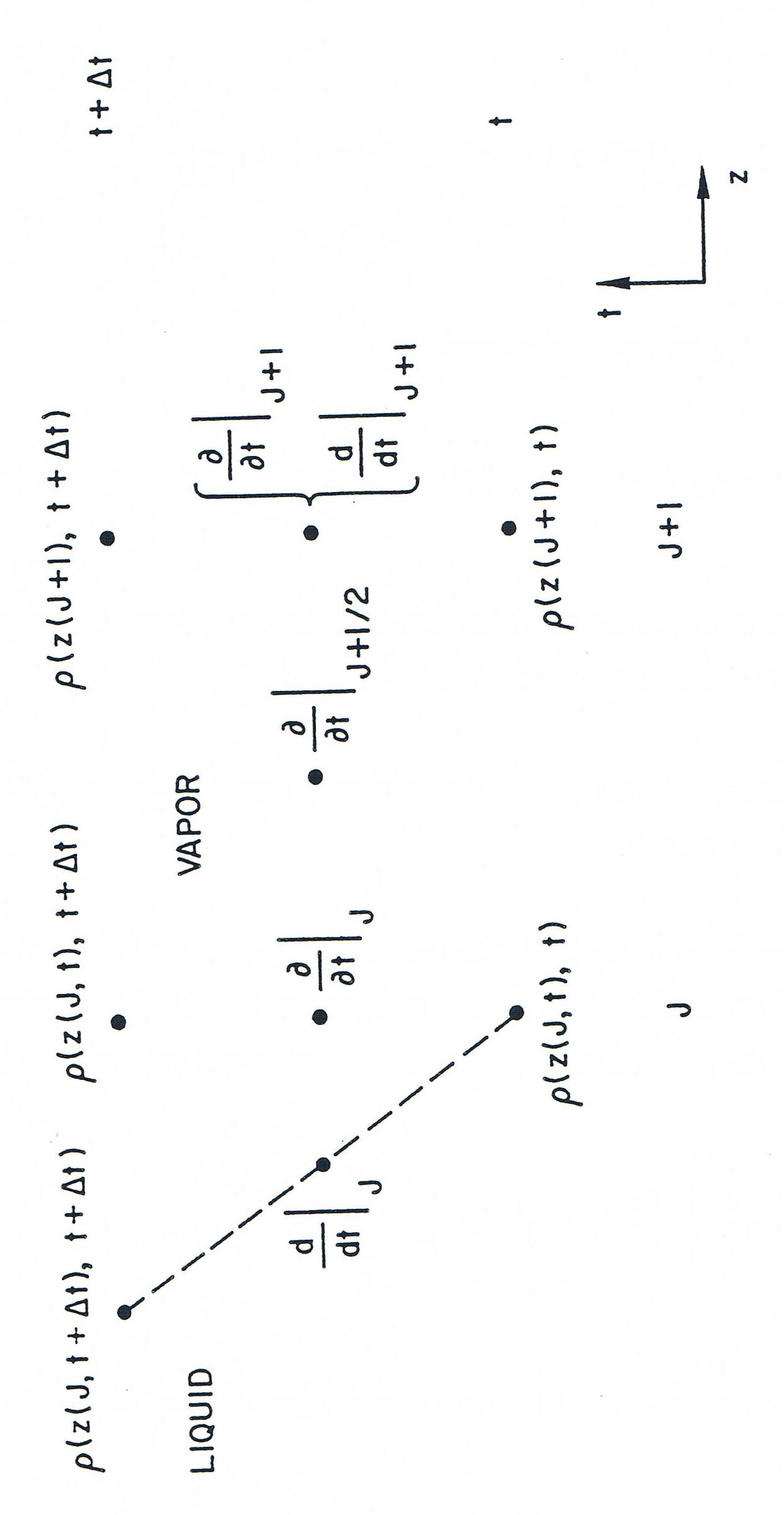
Figure 12.6.3 Evaluation of the total Derivative at a Liquid-Vapor Interface

so the partial derivative at $J$ is differenced as though the interface were stationary at $z\left(J,t\right)$. However, the interface is moving at a velocity $v^{i}$ and moves a distance $v^{i}\Delta t$ from $z\left(J,t\right)$ to $z\left(J,t + \Delta t\right)$ during the time step, so the spatial derivative in the continuity equation must be differenced from $z\left(J + 1,t + \Delta t\right)$ to $z\left(J, t + \Delta t\right)$, rather than to $z\left(J,t\right)$. Thus, the continuity equation for an interface node will involve advanced time quantities at three spatial points ($z \left(J,t \right)$, $z \left( J,t + \Delta t \right)$, and $z\left(J + 1, t + \Delta t\right)$) rather than at two. This difficulty can be resolved if the partial derivative with respect to time is expressed in terms of $\rho\left(z\left(J,t + \Delta t\right), t + \Delta t\right)$ rather than $\rho\left(z\left(J,t\right), t + \Delta t\right)$ by introducing the Lagrangian total derivative, $\frac{d\rho}{dt}$.

(12.6-48) $$\frac{d\rho}{dt} = \frac{\partial\rho}{\partial t} + v\frac{\partial\rho}{\partial z}$$

or

(12.6-49) $$\frac{\partial\rho}{\partial t} = \frac{d\rho}{dt} - v\frac{\partial\rho}{\partial z}$$

with

(12.6-50) $$\frac{d\rho}{dt} = \frac{\rho\left( z\left( J,t + \Delta t \right),t + \Delta t \right) - \rho\left( z\left( J,t \right),t \right) + \rho\left( z(J + 1),t + \Delta t \right) - \rho(z(J + 1),t)}{2\Delta t}$$

(12.6-51) $$v = \frac{v^{i}}{2}$$

and

(12.6-52) $$\frac{\partial\rho}{\partial z} = \frac{\rho\left( z\left( J,t + \Delta t \right),t + \Delta t \right) - \rho(z(J + 1),t + \Delta t)}{z\left( J,t + \Delta t \right) - z\left(J + 1, t + \Delta t \right)}$$

The factor of (1/2) appears in the velocity term to represent the average of the velocity of the interface point $J$ (which is $v^{i}$) and that of the point $J + 1$ (which is zero). This formulation is equivalent to expressing $\rho\left(z\left( J,t\right),t + \Delta t\right)$ as an interpolated value between $\rho\left(z\left(J,t + \Delta t\right)\right)$ and $\rho\left(z(J + 1), t + \Delta t\right)$. The continuity equation now takes the form

(12.6-53) $$\frac{\partial W}{\partial z} + A_{c}\frac{d\rho}{dt} - v\frac{\partial\rho}{\partial z} = A_{c}\frac{Q}{\lambda}$$

Let a node boundary quantity $x$ be represented at the lower interface by $x_{j}^{i}(J1)$ and at the upper interface by $x_{j}^{i}(J2)$ where $j = 1$ or $2$ to designate the beginning or end of the time step. A node midpoint quantity $y$ is represented at the lower interface by $y_{j}(J1)$ (since it is contained in node $J1$) and at the upper interface by $y_{j}(J2-1)$ (since it is located in node $J2-1$). As shown in Fig. 12.6-4, $J1$ is the number of the fixed mesh node boundary below the lower interface, while $J2$ is the fixed node boundary number above the upper interface. Looking first at the lower interface, the total time derivative of the density is then

(12.6-54) $$\frac{d\rho}{dt} = \frac{\rho_{2}(J1 + 1) - \rho_{1}(J1 + 1) + \rho_{2}^{i}(J1) - \rho_{1}^{i}(J1)}{2\Delta t}$$

or, using Eq. (12.6-22) and Eq. (12.6-37) to express $\frac{d\rho}{dt}$ in terms of the change in vapor pressure,

(12.6-55) $$\frac{d\rho}{dt} = \frac{1}{2\Delta t}\left(\Delta \rho(J1 + 1)\frac{d\rho}{dp_{J1 + 1}} + \Delta\rho^{i}(J1)\frac{d\rho^{i}}{dp_{J1}} \right)$$

The spatial derivative term becomes

(12.6-56) $$v\frac{\partial\rho}{\partial z} = \frac{v_{2}^{i}(J1)}{2}\frac{(\rho_{2}(J1 + 1) - \rho_{2}^{i}(J1))}{(z(J1 + 1) - z_{2}^{i}(J1))}$$

The advanced time velocity is expressed in the linearized form of Eq. (12.6-21) as

(12.6-57) $$v_{2}^{i}(J1) = v_{1}^{i}(J1) + \Delta v^{i}(J1)$$

It is apparent from Eq. (12.6-56) and Eq. (12.6-57) that the added complication of treating the bubble interface introduces two extra unknowns beyond those described in Section 12.6.2.1, namely, the change in interface velocity $\Delta v^{i}$ and the advanced time interface position $z_2^i$ (the current time interface velocity, $v_1^i$, is assumed known). As will be shown in Section 12.6.2.2.2 and Section 12.6.2.2.3, both of these quantities can be expressed as functions of $\Delta p$ and of known terms, so that their effect on the final differenced equation is to add terms to the coefficients $c_{1,J}$ and $c_{3,J}$ and to the source term $h_{J}$ in Eq. (12.6-45).

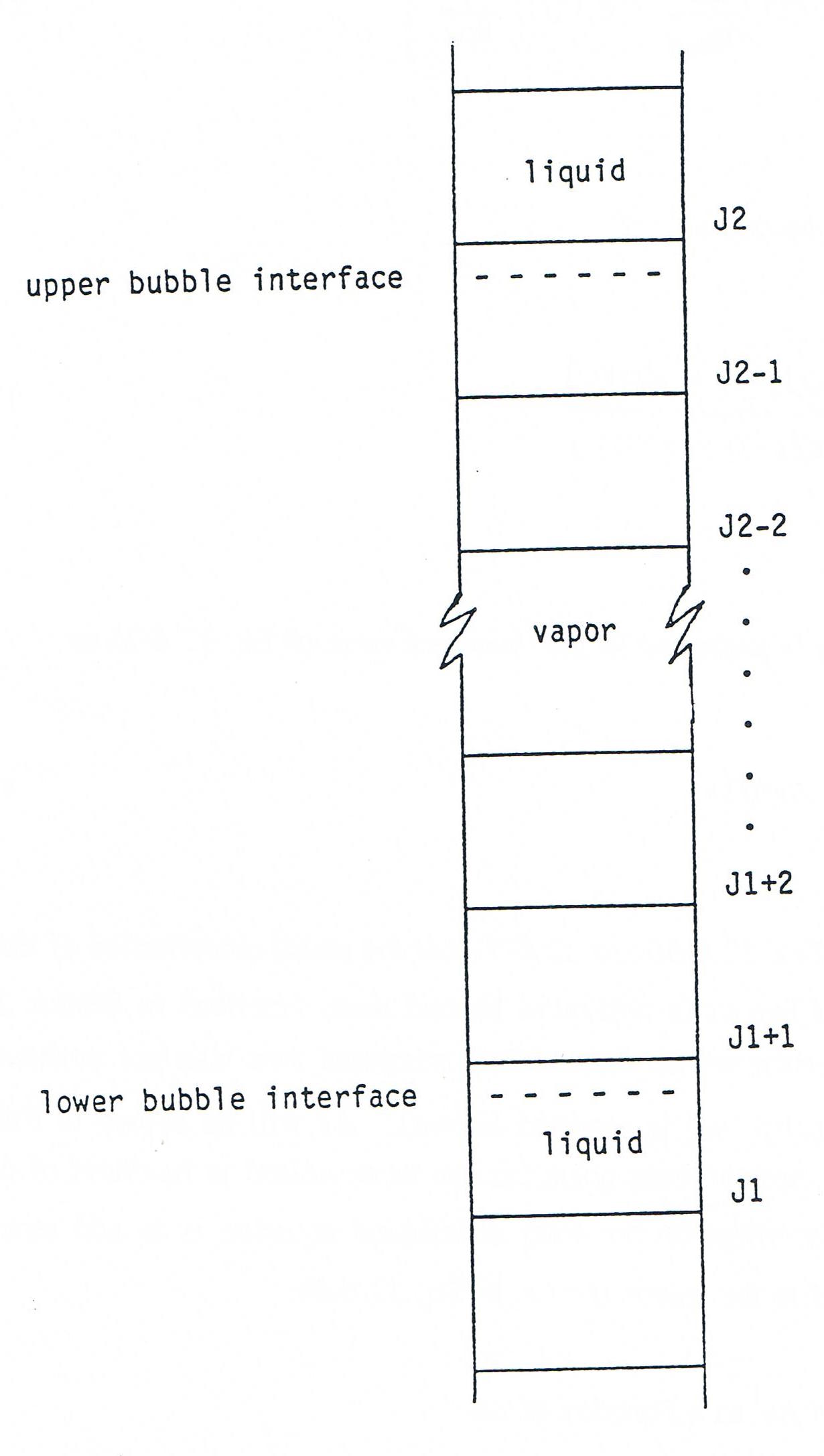
Figure 12.6.4 Placement of a Bubble in the SASSYS-1 Axial Coolant Mesh

12.6.2.2.2. Formulation of $\Delta v^i$ as a Function of $\Delta p$

If the bubble under consideration is labeled bubble $K$, the change in interface velocity is calculated from the change in mass flow rate $\Delta W_{l}\left(K\right)$ in liquid slug $K$, which is the slug below bubble $K$:

(12.6-58) $$\Delta v^{i}(J1) = \frac{\Delta W_{l}\left( K \right)}{\rho_{l}^{i}(J1)A_{c}(J1)}f_{rwt}(K)$$

where $f_{rwt}\left(K\right)$ is the liquid film rewetting factor at the top of slug $K$ and $\rho_{l}^{i}(J1)$ is the liquid sodium density at the interface. The film rewetting factor accounts for the effect of liquid film on the cladding and structure on the interface velocity; this has already been discussed in Section 12.3. From Eq. (12.3-6) of Section 12.3, the liquid film rewetting factor is

(12.6-59) $$f_{rwt} = \frac{v^{i}}{v_{l}} = \frac{1 - P_{e}\left( w_{fe}v_{fe} + \gamma_{2}w_{fs}v_{fs} \right)/(v_{l}A_{c})}{1 - P_{e}\left( w_{fe} + \gamma_{2}w_{fs} \right)/A_{c}}$$

The change in mass flow rate is computed from the liquid slug momentum equation given in Eq. (12.2-38):

(12.6-60) $$\Delta W_{l}\left( K \right) = \frac{\left( AA_{0}\left( K \right) + \theta_{2}\left( \Delta p_{b}\left( K \right) - \Delta p_{t}\left( K \right) \right) \right)\Delta t}{I_{1}\left( K \right) + \theta_{2}\Delta I_{1}\left( K \right) + BB_{0}\left( K \right)\theta_{2}\Delta t}$$

with $\theta_{1} = \theta_{2} = 1/2$ for the semi-implicit method and $\theta_{1} = 0$, $\theta_{2} = 1$ for the fully implicit formulation. The pressure changes are defined as

$\Delta p_{b}\left(K\right) =$ change in pressure at lower end of liquid slug K.

$\Delta p_{t}\left(K\right) =$ change in pressure at upper end of liquid slug K.

Since $\Delta p_{t}\left(K\right)$ is the pressure change at the bubble interface,

(12.6-61) $$\Delta p_{t}\left( K \right) = \Delta p^{i}(J1)$$

Therefore, $\Delta v^{i}(J1)$ can be split into two parts as

(12.6-62) $$\Delta v^{i}(J1) = \Delta v_{0}^{i}(J1) + \Delta p^{i}(J1)\frac{dv^{i}}{dp_{J1}}$$

with

(12.6-63) $$\Delta v_{0}^{i}(J1) = \frac{f_{fwt}(K)}{\rho_{l}^{i}(J1)A(J1)}\frac{\left( AA_{0}\left( K \right) + \theta_{2}\Delta p_{b}\left( K \right) \right)\Delta t}{I_{1}\left( K \right) + \theta_{2}\Delta I_{1}\left( K \right) + BB_{0}\left( K \right)\theta_{2}\Delta t}$$

being the change in interface velocity with no change in interface pressure and

(12.6-64) $$\frac{dv^{i}}{dp_{J1}} = - \frac{f_{rwt}\left( K \right)}{\rho_{l}^{i}(J1)A(J1)}\frac{\theta_{2}\Delta t}{I_{1}\left( K \right) + \theta_{2}\Delta I_{1}\left( K \right) + BB_{0}\left( K \right)\theta_{2}\Delta t}$$

being the velocity change with respect to the change in interface pressure. With the change in interface velocity now expressed as a linear function of the change in interface pressure Eq. (12.6-62), the advanced time interface velocity in the expression for the spatial derivative term $v\frac{\partial\rho}{\partial z}$ Eq. (12.6-56) can be replaced using Eq. (12.6-57) and Eq. (12.6-62). In addition, the advanced time densities in Eq. (12.6-56) can be linearized through Eq. (12.6-22) and written in terms of pressure changes form Eq. (12.6-37). This gives $v\frac{\partial\rho}{\partial z}$ as

(12.6-65) $$\begin{split}v\frac{\partial\rho}{\partial z} = \frac{1}{2}\left( v_{1}^{i}(J1) + \Delta v_{0}^{i}(J1) + \Delta p_{i}(J1)\frac{dv^{i}}{dp_{J1}} \right) \\ \times \frac{\rho_{i}(J1 + 1) + \Delta p(J1 + 1)\frac{d\rho}{dp_{J1 + 1}} - \rho_{1}^{i}(J1) - \Delta p^{i}(J1)\frac{d\rho^{i}}{dp_{J1}}}{z(J1+1) - z_2^i(J1)}\end{split}$$

Now, all that remains is to express the interface position $z_{2}^{i}$ as a function of the change in pressure; this will be done in the next subsection.

12.6.2.2.3. Formulation of $z_2^i$ as a Function of $\Delta p$

The function height can be written as

(12.6-66) $$z_{2}^{i}(J1) = z_{1}^{i}(J1) + \frac{\Delta t}{2}\left( v_{1}^{i}(J1) + v_{2}^{i}(J1) \right)$$

which, substituting Eq. (12.6-57) and Eq. (12.6-62) for $v_{2}^{i}$, becomes

(12.6-67) $$\begin{align}\begin{aligned}z_{2}^{i}(J1) &= z_{1}^{i}(J1) + \frac{\Delta t}{2}v_{1}^{i}(J1) + \left( v_{1}^{i}(J1) + \Delta v_{0}^{i}(J) + \Delta p^{i}(J1)\frac{dv^{i}}{dp_{J1}} \right)\\&= z_{1}^{i}(J1) + v_{1}^{i}(J1)\Delta t + \frac{\Delta t}{2}v_{0}^{i}(J1) + \Delta p^{i}(J1)\frac{\Delta t}{2}\frac{dv^{i}}{dp_{J1}}\end{aligned}\end{align}$$

Define

(12.6-68) $$z_{0}^{i}(J1) = z_{1}^{i}(J1) + v_{1}^{i}(J1)\Delta t + \frac{\Delta t}{2}\Delta v_{0}^{i}(J1)$$

as the interface height with no pressure change at the interface and

(12.6-69) $$\frac{dz^{i}}{dp_{J1}} = \frac{1}{2}\Delta t\frac{dv^{i}}{dp_{J1}}$$

as the change in interface height with respect to the change in interface pressure. Then $z_{2}^{i}$ is the linear function

(12.6-70) $$z_{2}^{i}(J1) = z_{0}^{i}(J1) + \Delta p^{i}(J1)\frac{dz^{i}}{dp_{J1}}$$

Using Eq. (12.6-70) in Eq. (12.6-65), $v\frac{\partial\rho}{\partial z}$ can be expressed as a function of only $\Delta p$,

(12.6-71) $$\begin{split}v\frac{\partial \rho}{\partial z} = \frac{1}{2}\left( v_{1}^{i}(J1) + \Delta v_{0}^{i}(J1) + \Delta p^{i}(J1)\frac{dv^{i}}{dp_{J1}} \right) \\ \times \frac{\rho_{1}(J1 + 1) + \Delta p(J1 + 1)\frac{d\rho}{dp_{J1 + 1}} - \rho_1^i(J1) - \Delta p^i\frac{d\rho^i}{dp_{J1}}}{z(J1 + 1) - z_{0}^{i}(J1) - \Delta p^{i}(J1)\frac{dz^{i}}{dp_{J1}}}\end{split}$$

12.6.2.2.4. Final Differenced Form of the Continuity Equation at the Lower Interface as a Function of Only $\Delta p$ and $\Delta W$

With $\frac{d\rho}{dt}$ in the interface continuity equation, Eq. (12.6-53), written in the form in Eq. (12.6-55) and $v\frac{\partial\rho}{\partial z}$ given by Eq. (12.6-71) and all other terms in Eq. (12.6-53) treated as in Section 12.6.2.1, the differenced form of the continuity equation at the lower interface is, after multiplication by $\left( z(J1 + 1) - z_{2}^{i}(J1) \right)$ and substitution of Eq. (12.6-70) for $z_{2}^{i}$,

(12.6-72) $$\begin{split}\Delta t\left( W_{1}(J1 + 1) - W_{1}^{i}(J1) + \Delta W(J1 + 1) - \Delta W^{i}(J1) \right) \\ + \frac{A_{c}(J1)}{2}\left( \Delta \rho(J1 + 1)\frac{d\rho}{dp_{J1 + 1}} + \Delta \rho^{i}(J1)\frac{d\rho^{i}}{dp_{J1}} \right)\bigg( z(J1 + 1) - z_{0}^{i}(J1) \\ - \Delta p^{i}(J1)\frac{dz^{i}}{dp_{J1}} \bigg) - \frac{A_{c}(J1)\Delta t}{2}\left( v_{1}^{i}(J1) + \Delta v_{0}^{i}(J1) + \Delta p^{i}(J1)\frac{dv^{i}}{dp_{J1}} \right) \\ \times \left( \rho_{1}(J1 + 1) + \Delta p(J1 + 1)\frac{d\rho}{dp_{J1 + 1}} - \rho_{1}^{i}(J1) - \Delta p^{i}(J1)\frac{d\rho^{i}}{dp_{J1}} \right) \\ = A_{c}(J1)\Delta t\frac{Q_{0}(J1)}{\lambda_{1}(J1)}\bigg[ 1 + \left( \Delta p^{i}(J1)\frac{dT^{i}}{dp_{J1}} + \Delta p(J1 + 1)\frac{dT}{dp_{J1 + 1}} \right)\frac{1}{2Q_{0}(J1)}\frac{dQ_{0}}{dT_{J1}} \\ - \left( \Delta p^{i}(J1) + \Delta p(J1 + 1)\frac{1}{2\lambda_{1}(J1)}\frac{d\lambda}{dp_{J1}} \right) \bigg]\bigg( z(J1 + 1) - z_{0}^{i}(J1) \\ + \Delta p^{i}(J1)\frac{dz^{i}}{dp_{J1}} \bigg)\end{split}$$

Setting $\Delta z_{0}(J1) = z(J1 + 1) - z_{0}^{i}(J1)$ and eliminating second-order terms gives a differenced interface continuity equation which is linear in the pressure and mass flow rate changes:

(12.6-73) $$\begin{split}\Delta t\left( W_{1}(J + 1) - W_{1}^{i}(J1) + \Delta W(J1 + 1) - \Delta W^{i}(J1) \right) \\ + \frac{A_{c}(J1)}{2}\Delta z_{0}(J1)\left( \Delta p(J1 + 1)\frac{d\rho}{dp_{J1 + 1}} + \Delta p^{i}(J1)\frac{d\rho^{i}}{dp_{J1}} \right) \\ - \frac{A_{c}(J1)\Delta t}{2} \bigg\{ \left\lbrack v_{1}^{i}(J1) + \Delta v_{0}^{i}(J1) \right\rbrack\left\lbrack \rho_{1}(J1 + 1) - \rho_{1}^{i}(J1) \right\rbrack \\ + \left[v_{1}^{i}(J1) + \Delta v_{0}^{i}(J1) \right] \left\lbrack \Delta p(J1 + 1)\frac{d\rho}{dp_{J1 + 1}} - \Delta p^{i}(J1)\frac{d\rho^{i}}{dp_{J1}} \right\rbrack \\ + \Delta p^{i}(J1)\frac{dv^{i}}{dp_{J1}}\left\lbrack \rho_{1}(J1 + 1) - \rho_{1}^{i}(J1) \right\rbrack \bigg\} - A_{c}(J1)\Delta t\frac{Q_{0}(J1)}{\lambda_{1}(J1)} \bigg\{ \Delta z_{0}(J1) \\ - \Delta p^{i}(J1)\frac{dz^{i}}{dp_{J1}} + \Delta z_{0}(J)\left\lbrack \Delta p^{i}(J1)\frac{dT^{i}}{dp_{J1}} + \Delta p(J1 + 1)\frac{dT}{dp_{J1 + 1}} \right\rbrack\frac{1}{2Q_{0}(J1)}\frac{dQ_{0}}{dT_{J1}} \\ - \Delta z_{0}(J1)\frac{1}{2\lambda_{1}(J1)}\left\lbrack \Delta p^{i}(J1) + \Delta p(J1 + 1) \right\rbrack\frac{d\lambda}{dp_{J1}} \bigg\} = 0\end{split}$$

Eq. (12.6-73) can be simplified by defining the coefficients

(12.6-74) $$\begin{split}c_{1,J1} = \frac{A_{c}(J1)}{2}\bigg\{\Delta z_{0}(J1)\frac{d\rho^{i}}{dp_{J1}} + \Delta t\bigg[ \left( v_{1}^{i}(J1) + \Delta v_{0}^{i}(J1) \right)\frac{d\rho^{i}}{dp_{J1}} \\ - \left( \rho_{1}(J1 + 1) - \rho_{1}^{i}(J1) \right)\frac{dv^{i}}{dp_{J}} \bigg] + \Delta t\bigg[ \frac{2Q_{0}(J1)}{\lambda_{1}(J1)}\frac{dz^{i}}{dp_{J1}} \\ - \frac{\Delta z_{0}(J1)}{\lambda_{1}(J1)}\frac{dQ_{0}}{dT_{J1}}\frac{dT^{i}}{dp_{J1}} + \frac{Q_{0}(J1)\Delta z_{0}(J1)}{\lambda_{1}^{2}(J1)}\frac{d\lambda}{dp_{J1}} \bigg]\bigg\}\end{split}$$

(12.6-75) $$c_{2,J1} = - \Delta t$$

(12.6-76) $$\begin{split}c_{3,J1} = \frac{A_{c}(J1)}{2}\bigg\{\Delta z_{0}(J1)\frac{d\rho}{dp_{J1 + 1}} - \Delta t \left( v_{1}^{i}(J1) + \Delta v_{0}^{i}(J1) \right)\frac{d\rho}{dp_{J1 + 1}} \\ - \Delta t\frac{\Delta z_{0}(J1)}{\lambda_{1}(J1)}\left\lbrack \frac{dQ_{0}}{dT_{J1}}\frac{dT}{dp_{J1 + 1}} - \frac{Q_{0}(J1)}{\lambda_{1}(J1)}\frac{d\lambda}{dp_{J1}} \right\rbrack \bigg\}\end{split}$$

(12.6-77) $$c_{4,J1} = \Delta t$$

and the source term

(12.6-78) $$\begin{split}h_{J1} = \Delta t \bigg\{ W_{1}^{i}(J1) - W_{1}(J1 + 1) + A_{c}(J1) \bigg[\frac{1}{2}\big( v_{1}^{i}(J1) \\ + \Delta v_{0}^{i}(J1) \big)\left( \rho_{1}(J1 + 1) - \rho_{1}^{i}(J1) \right) + \frac{Q_{0}(J1)\Delta z_{0}(J1)}{\lambda_{1}(J1)} \bigg]\bigg\}\end{split}$$

Then the differenced continuity equation at the lower interface can be written as

(12.6-79) $$c_{1,J1}\Delta p^{i}(J1) + c_{2,J1}\Delta W^{i}(J1) + c_{3,J1}\Delta p(J1 + 1) + c_{4,J1}\Delta W(J1 + 1) = h_{J1}$$

Note that with $v_{1}^{i}$, $\Delta v_{0}^{i}$, $\frac{dv^{i}}{dp}$, and $\frac{dz^{i}}{dp}$ set to zero, the expressions for the coefficients $c_{1,J1}$, and the source term $h_{J1}$ reduce to the forms given at the end of Section 12.6.2.1 for the continuity equation for a mesh segment which lies entirely within the bubble.

12.6.2.2.5. Differenced Form of the Continuity Equation at the Upper Interface

The derivation of the differenced continuity equation at the upper interface is nearly identical to that for the lower interface, and so just a brief explanation will be given here. The terms in the interface continuity equation of Eq. (12.6-53) are now expressed as follows:

The time derivative is

(12.6-80) $$\begin{align}\begin{aligned}\frac{d\rho}{dt} &= \frac{\rho_{2}^{i}(J2) - \rho_{1}^{i}(J2) + \rho_{2}(J2 - 1) - \rho_{1}(J2 - 1)}{2\Delta t}\\&= \frac{1}{2\Delta t}\left( \Delta p^{i}(J2)\frac{d\rho^{i}}{dp_{J2}} + \Delta p(J2 - 1)\frac{d\rho}{dp_{J2 - 1}} \right)\end{aligned}\end{align}$$

The $v\frac{\partial\rho}{\partial z}$ term is

(12.6-81) $$v\frac{\partial\rho}{\partial z} = \frac{v_{1}^{i}(J2) + \Delta v^{i}(J2)}{2}\frac{\rho_{2}^{i}(J2) - \rho_{2}(J2 - 1)}{z_{2}^{i}(J2) - z(J2 - 1)}$$

where

(12.6-82) $$\Delta v^{i}(J2) = \frac{\Delta W_{l}\left( K + 1 \right)}{\rho_{l}^{i}(J2)A_{c}(J2 - 1)}f_{rwb}(K + 1)$$

and

(12.6-83) $$\Delta W_{l}\left( K + 1 \right) = \frac{\left( AA_{0}\left( K + 1 \right) + \theta_{2}\left( \Delta p^{i}(J2) - \Delta p^{i}\left( K + 1 \right) \right) \right)\Delta t}{I_{1}\left( K + 1 \right) + \theta_{2}\Delta I_{1}\left( K + 1 \right) + BB_{0}\left( K + 1 \right)\theta_{2}\Delta t}$$

The rewetting factor at the bottom of liquid slug $K + 1$, $f_{rwb}\left(K + 1\right)$, is computed as in Eq. (12.6-59). The expression for $\Delta v_{i}(J2)$ then reduces to

(12.6-84) $$\Delta v^{i}(J2) = \Delta v_{0}^{i}(J2) + \Delta p^{i}(J2)\frac{dv^{i}}{dp_{J2}}$$

with the definitions of $\Delta v_{0}^{i}(J2)$ and $\frac{dv^{i}}{dp_{J2}}$ being set as were those for $\Delta v_{0}^{i}(J1)$ and $\frac{dv^{i}}{dp_{J1}}$. Also,

(12.6-85) $$z_{2}^{i}(J2) = z_{0}^{i}(J2) + \Delta p^{i}(J2)\frac{dz^{i}}{dp_{J2}}$$

can be derived in exactly the same fashion as was Eq. (12.6-70). Therefore,

(12.6-86) $$\begin{split}v\frac{\partial\rho}{\partial z} = \frac{1}{2}\left( v_{1}^{i}(J2) + \Delta v_{0}^{i}(J2) + \Delta p^{i}(J2)\frac{dv^{i}}{dp_{J2}} \right) \\ \times \left( \frac{\rho_{1}^{i}(J2) + \Delta p^{i}(J2)\frac{d\rho^{i}}{dp_{J2}} - \rho_{1}^{i}(J2 - 1) - \Delta p(J2 - 1)\frac{d\rho}{dp_{J2 - 1}}}{z_{0}^{i}(J2) + \Delta p^{i}(J2)\frac{dz^{i}}{dp_{J2}} - z(J2 - 1)} \right)\end{split}$$

Substituting Eq. (12.6-80) and Eq. (12.6-86) into Eq. (12.6-53) and expressing $\frac{\partial W}{\partial z}$ and $A_{c}\frac{Q}{\lambda}$ as in Section 12.6.2.1 gives the differenced upper interface continuity equation

(12.6-87) $$\begin{split}c_{1,J2 - 1}\Delta p(J2 - 1) + c_{2,J2 - 1}\Delta W(J2 - 1) + c_{3,J2 - 1}\Delta p^{i}(J2) \\ + c_{4,J2 - 1}\Delta W^{i}(J2) = h_{J2 - 1}\end{split}$$

where

(12.6-88) $$\begin{split}c_{1,J2 - 1} = \frac{A_{c}(J2 - 1)}{2}\bigg\{\Delta z_{0}(J2 - 1)\frac{d\rho}{dp_{J2 - 1}} + \Delta t\bigg[\left( v_{1}^{i}(J2) + \Delta v_{0}^{i}(J2) \right)\frac{d\rho}{dp_{J2 - 1}} \\ + \frac{\Delta z_{0}(J2 - 1)}{\lambda_{1}(J2 - 1)}\left(\frac{dQ_{0}}{dT_{J2 - 1}}\frac{dT}{dp_{J2 - 1}} - \frac{Q_{0}(J2 - 1)}{\lambda(J2 - 1)}\frac{d\lambda}{dp_{J2}} \right) \bigg] \bigg\}\end{split}$$

(12.6-89) $$c_{2,J2 - 1} = - \Delta t$$

(12.6-90) $$\begin{split}c_{3,J2 - 1} = \frac{A_{c}(J2 - 1)}{2}\Bigg\{\Delta z_{0}(J2 - 1)\frac{d\rho^{i}}{dp_{J2}} - \Delta t\Bigg[\left( v_{1}^{i}(J2) + \Delta v_{0}^{i}(J2) \right)\frac{d\rho^{i}}{dp_{J2}} \\ + \left\lbrack \rho_{1}^{i}(J2) - \rho_{1}(J2 - 1) \right\rbrack\frac{dv^{i}}{dp_{J2}}\Bigg] - \Bigg[\Delta t\frac{2Q_{0}(J2 - 1)}{\lambda_{1}(J2 - 1)}\frac{dz^{i}}{dp_{J2}} \\ + \frac{\Delta z_{0}(J2 - 1)}{\lambda_{1}(J2 - 1)}\left(\frac{dQ_{0}}{dT_{J2 - 1}}\frac{dT^{i}}{dp_{J2}} - \frac{Q_{0}(J2 - 1)}{\lambda_{1}(J2 - 1)}\frac{d\lambda}{dp_{J2}}\right)\Bigg]\Bigg\}\end{split}$$

(12.6-91) $$c_{4,J2 - 1} = \Delta t$$

(12.6-92) $$\begin{split}h_{J2 - 1} = \Delta t\bigg\{ W_{1}(J2 - 1) - W_{1}^{i}(J2) + A_{c}(J2 - 1)\bigg[\frac{1}{2}( v_{1}^{i}(J2) \\ + \Delta v_{0}^{i}(J2))\left( \rho_{1}^{i}(J2) - \rho_{1}(J2 - 1) \right) + \frac{Q_{0}(J2 - 1)\Delta z_{0}(J2 - 1)}{\lambda_{1}(J2 - 1)}\bigg]\bigg\}\end{split}$$

and

(12.6-93) $$\Delta z_{0}(J2 - 1) = z_{1}^{i}(J2) - z(J2 - 1)$$

12.6.2.3. Finite Differencing of the Momentum Equation for a Mesh Segment Contained Entirely in One Bubble

Now that differenced forms of the continuity equation both within the bubble and at liquid-vapor interfaces have been derived, a similar process must be applied in the momentum equation. The differencing of the momentum equation is accomplished in essentially the same way as that of the continuity equation. Once again, bubble interface will be ignored for the sake of simplicity until the equations for an interior node have been developed.

12.6.2.3.1. Differencing of the Momentum Equation

The differenced forms of the terms in the momentum equation, Eq. (12.6-2), are a follows. The channel pressure drop is given by

(12.6-94) $$\frac{\partial p}{\partial z}\Big|_{J + \frac{1}{2}} = \frac{p_{2}(J + 1) - p_{2}(J)}{z(J + 1) - z(J)}$$

The momentum convection takes the form

(12.6-95) $$\left. \frac{1}{A_{c}}\frac{\partial}{\partial z}\left( \frac{W^{2}}{\rho A_{c}} \right) \right|_{J + \frac{1}{2}} = \frac{1}{A_{c}^{2}(J)\left( z(J + 1) - z(J) \right)}\left( \frac{W_{2}^{2}(J + 1)}{\rho_{2}(J + 1)} - \frac{W_{2}^{2}(J)}{\rho_{2}(J)} \right)$$

The condensation term is expressed in terms of the contributions from cladding and structure as

(12.6-96) $$F_{c}(J) = F_{ce}(J) + F_{cs}(J)$$

where the functions for $F_{ce}$ and $F_{cs}$ are linearly approximated as follows:

(12.6-97) $$\text{if }Q_{e_{2}}(J) \geq 0,\ F_{ce}(J) = 0$$

(12.6-98) $$\text{if }Q_{e_{2}}(J) < 0,\ F_{ce}(J) = \frac{Q_{e_{2}}(J)}{2\lambda_{2}(J)A_{c}(J)}\left( \frac{W_{2}(J)}{\rho_{2}(J)} + \frac{W_{2}(J + 1)}{\rho_{2}(J + 1)} \right)$$

and

(12.6-99) $$\text{if }Q_{s_{2}}(J) \geq 0,\ F_{cs}(J) = 0$$

(12.6-100) $$\text{if }Q_{s_{2}}(J) \leq 0,\ F_{cs}(J) = \frac{Q_{s_{2}}(J)}{2\lambda_{2}(J)A_{c}(J)}\left( \frac{W_{2}(J)}{\rho_{2}(J)} + \frac{W_{2}(J + 1)}{\rho_2(J + 1)} \right)$$

$Q_{e_2}(J)$ and $Q_{s_2}(J)$ are defined in Eq. (12.6-19). Now, linearize $Q_{e_2}$ and $Q_{s_2}$ by defining

(12.6-101) $$Q_{oe}(J) = \gamma(J) \frac{T_{e_{2}}(J) - \overline{T}_{1}\left(1\right)}{R_{ec_2}(J)}$$

(12.6-102) $$\frac{dQ_{oe}}{dT_{J}} = -\frac{\gamma(J)}{R_{ec_2}(J)}$$

(12.6-103) $$Q_{os}(J) = \gamma(J)\gamma_{2}(J)\frac{T_{s_{2}}(J) - {\overline{T}}_{1}(J)}{R_{sc_{2}}(J)}$$

(12.6-104) $$\frac{dQ_{os}}{dT_{J}} = - \frac{\gamma(J)\gamma_{2}(J)}{R_{sc_{2}}(J)}$$

These expressions are related to $Q_{o}(J)$, defined in Section 12.6.2.1.2, by

(12.6-105) $$Q_{o}(J) = Q_{oe}(J) + Q_{os}(J)$$

and

(12.6-106) $$\frac{dQ_{o}}{dT_{J}} = \frac{dQ_{oe}}{dT_{J}} + \frac{dQ_{os}}{dT_{J}}$$

Substituting these functions into the above formulations of $F_{ce}$ and $F_{cs}$ gives

(12.6-107) $$\text{if }Q_{e_{2}}(J) \geq 0,\ F_{ce}(J) = 0$$

(12.6-108) $$\begin{split} \text{if }Q_{e_{2}}(J) < 0,\ F_{ce}(J) = \frac{1}{2\lambda_{2}(J)A_{c}(J)}\left( \frac{W_{2}(J)}{\rho_{2}(J)} + \frac{W_{2}(J + 1)}{\rho_{2}(J + 1)} \right) \\ \times \left[ Q_{oe}(J) + \frac{1}{2}\frac{dQ_{oe}}{dT_{J}}\left( \Delta T(J) + \Delta T(J + 1) \right) \right]\end{split}$$

(12.6-109) $$\text{if } Q_{s_{2}}(J) \geq 0,\ F_{cs}(J) = 0$$

(12.6-110) $$\begin{split} \text{if }Q_{s_{2}}(J) < 0,\ F_{cs}(J) = \frac{1}{2\lambda_{2}(J)A_{c}(J)}\left( \frac{W_{2}(J)}{\rho_{2}(J)} + \frac{W_{2}(J + 1)}{\rho_{2}(J + 1)} \right) \\ \times \left[ Q_{os}(J) + \frac{1}{2}\frac{dQ_{os}}{dT_J}\left( \Delta T(J) + \Delta T(J+1) \right) \right]\end{split}$$

If the definitions

(12.6-111) $$\begin{split}F_{oe}(J) = \begin{cases} 0 & Q_{e_{2}} \geq 0 \\ Q_{oe}(J) & Q_{e_{2}}(J) < 0 \end{cases}\end{split}$$

(12.6-112) $$\begin{split}F_{os}(J) = \begin{cases} 0 & Q_{s_{2}} \geq 0, \\ Q_{os}(J) & Q_{s_{2}}(J) < 0 \end{cases}\end{split}$$

(12.6-113) $$F_{o}(J) = F_{oe}(J) + F_{os}(J)$$

are used in the expressions for $F_{ce}$ and $F_{cs}$, the condensation term becomes

(12.6-114) $$\begin{split}F_{c}(J) = \frac{F_{o}(J)}{2A_{c}(J)\lambda_{2}(J)}\bigg[ 1 + \left( \frac{F_{oc}(J)}{2Q_{oe}(J)F_{o}(J)}\frac{dQ_{oe}}{dT_{J}} + \frac{F_{os}(J)}{2Q_{os}(J)F_{o}(J)}\frac{dQ_{os}}{dT_{J}} \right) \\ \times(\Delta t(J) + \Delta T(J + 1))\bigg]\left(\frac{W_{2}(J)}{\rho_{2}(J)} + \frac{W_{2}(J + 1)}{\rho_{2}(J + 1)} \right)\end{split}$$

This expression can be simplified by setting

(12.6-115) $$\begin{split}\frac{dF_{oe}}{dT_{J}} = \Bigg\{ \begin{cases} 0 & Q_{e_{2}}(J) \geq 0 \\ \frac{dQ_{oe}}{dT_{J}} & Q_{e_{2}}(J) < 0 \end{cases}\end{split}$$

which can be stated more compactly as

(12.6-116) $$\frac{dF_{oe}}{dT_{J}} = \frac{F_{oe}(J)}{Q_{oe}(J)}\frac{dQ_{oe}}{dT_{J}}$$

Similarly,

(12.6-117) $$\frac{dF_{os}}{dT_{J}} = \frac{F_{os}(J)}{Q_{os}(J)}\frac{dQ_{os}}{dT_{J}}$$

so that the definition

(12.6-118) $$\frac{dF_{o}}{dT_{J}} = \frac{dF_{oe}}{dT_{J}} + \frac{dF_{os}}{dT_{J}}$$

can be made. This gives

(12.6-119) $$\begin{split}F_{c}(J) = \frac{F_{o}(J)}{2A_{c}(J)\lambda_{2}(J)}\left\lbrack 1 + \frac{dF_{o}}{2F_{o}(J)}\frac{dF_{o}}{dT_{J}}\left( \Delta T(J) + \Delta T(J + 1) \right) \right\rbrack \\ \times\left( \frac{W_{2}(J)}{\rho_{2}(J)} + \frac{W_{2}(J + 1)}{\rho_{2}(J + 1)} \right)\end{split}$$

as the differenced form of the condensation term.

The change in mass flow rate with time is

(12.6-120) $$\frac{\partial W}{\partial t} = \frac{W_{2}(J) + W_{2}(J + 1) - W_{1}(J) - W_{1}(J + 1)}{2\Delta t}$$

The orifice pressure drop becomes

(12.6-121) $$\begin{split}\frac{W\left| W \right|}{2\rho_{v}A_{c}^{2}}\frac{\partial k_{or}}{\partial z} = \frac{1}{4A_{c}^{2}(J)}\left( \frac{W_{2}(J)\left| W_{2}(J) \right|}{\rho_{2}(J)} + \frac{W_{2}(J + 1)\left| W_{2}(J + 1) \right|}{\rho_{2}(J + 1)} \right) \\ \times\frac{k_{or}(J)}{z(J + 1) - z(J)}\end{split}$$

Finally, if the friction factor

(12.6-122) $$f_{v} = A_{fr}\left( \frac{D_{h}W}{\mu A_{c}} \right)^{b_{fr}}$$

is considered in the differencing, the friction term may be written as

(12.6-123) $$\begin{split}\frac{f_{v}W\left| W \right|}{2\rho A_{c}^{2}D_{h}} = \frac{A_{fr}W\left| W \right|^{1 + b_{fr}}}{2\rho\mu^{b_{fr}}D_{h}^{1 - b_{fr}}A_{c}^{2 + b_{fr}}} \\ = \frac{A_{fr}}{4D_h^{1-b_{fr}}(J)A_c^{2+b_{fr}}(J)}\left[ \frac{W_{2}(J+1)\left|W_{2}(J+1)\right|^{1+b_{fr}}}{\rho_{2}(J+1)\mu_2^{b_{fr}}(J+1)} + \frac{W_{2}(J)\left|W_{2}(J)\right|^{1+b_{fr}}}{\rho_{2}(J)\mu_2^{b_{fr}}(J)}\right]\end{split}$$

Using Eq. (12.6-94), Eq. (12.6-95), Eq. (12.6-119), Eq. (12.6-120), Eq. (12.6-121), and Eq. (12.6-123) results in a differenced momentum equation as follows:

(12.6-124) $$\begin{split}\frac{p_{2}(J + 1) - p_{2}(J)}{z(J + 1) - z(J)} + \frac{1}{A_{c}^{2}(J)\left( z(J + 1) - z(J) \right)}\left( \frac{W_{2}^{2}(J + 1)}{\rho_{2}(J + 1)} - \frac{W_{2}^{2}(J)}{\rho_{2}(J)} \right) \\ + \frac{A_{fr}}{4D_{h}^{1 - b_{fr}}(J)A_{c}^{2 + b_{fr}}(J)}\left\lbrack \frac{W_{2}(J + 1)\left| W_{2}(J + 1) \right|^{1 + b_{fr}}}{\rho_{2}(J + 1)\mu_{2}^{b_{fr}}(J + 1)} + \frac{W_{2}(J)\left| W_{2}(J) \right|^{1 + b_{fr}}}{\rho_{2}(J)\mu_{2}^{b_{fr}}(J)} \right\rbrack \\ - \frac{F_{o}(J)}{2A_{c}(J)\lambda_{2}(J)}\left\lbrack 1 + \frac{1}{2F_{o}(J)}\frac{dF_{o}}{dT_{J}}\left( \Delta T(J) + \Delta T(J + 1) \right) \right\rbrack\left( \frac{W_{2}(J)}{\rho_{2}(J)} + \frac{W_{2}(J + 1)}{\rho_{2}(J + 1)} \right) \\ + \frac{W_{2}(J) + W_{2}(J + 1) - W_{1}(J) - W_{1}(J + 1)}{2A_{c}(J)\Delta t} + \frac{1}{4A_{c}^{2}(J)}\Big( \frac{W_{2}(J)\left| W_{2}(J) \right|}{\rho_{2}(J)} \\ + \frac{W_{2}(J + 1)|W_{2}(J + 1)|}{\rho_{2}(J + 1)} \Big)\frac{k_{or}(J)}{z(J + 1) - z(J)} = 0\end{split}$$

The equation must now be linearized and reduced to a linear function of $\Delta p$ and $\Delta W$; this procedure will be discussed in the next subsection.

12.6.2.3.2. Linearization of Advanced Time Quantities and Introduction of Saturation Conditions

Eq. (12.6-124) is made linear by expressing the advanced time variables in linearized form as in Eq. (12.6-21). This means that, in addition to using the expressions in Eq. (12.6-22) through Eq. (12.6-25) for density, heat of vaporization, mass flow rate, and temperature, the linearized form of Eq. (12.6-124) must include the following representations of pressure and viscosity:

(12.6-125) $$p_{2}(J) = p_{1}(J) + \Delta p(J)$$

(12.6-126) $$\mu_{2}(J) = \mu_{1}(J) + \Delta\mu(J)$$

The differenced momentum equation therefore becomes

(12.6-127) $$\begin{split}\frac{p_{1}(J + 1) + \Delta p(J + 1) - p_{1}(J) - \Delta p(J)}{z(J + 1) - z(J)} + \frac{1}{A_{c}^{2}(J)\left( z(J + 1) - z(J) \right)} \\ \times\left( \frac{\left( W_{1}(J + 1) + \Delta W(J + 1) \right)^{2}}{\rho_{1}(J + 1) + \Delta\rho(J + 1)} - \frac{\left( W_{1}(J) + \Delta W(J) \right)^{2}}{\rho_{1}(J) + \Delta\rho(J)} \right) \\ + \frac{A_{fr}}{4D_{h}^{1 - b_{fr}}(J)A_{c}^{2 + b_{fr}}(J)}\Bigg( \frac{\left( W_{1}(J + 1) + \Delta W(J + 1) \right)\left| W_{1}(J + 1) + \Delta W(J + 1) \right|^{1 + b_{fr}}}{\left( \rho_{1}(J + 1) + \Delta\rho(J + 1) \right)\left( \mu_{1}(J + 1) + \Delta\mu(J + 1) \right)^{b_{fr}}} \\ + \frac{\left( W_{1}(J) + \Delta W(J) \right) \left| W_{1}(J) + \Delta W(J) \right|^{1 + b_{fr}}}{(\rho_{1}(J) + \Delta\rho(J)\left( \mu_{1}(J) + \Delta\mu(J) \right)^{b_{fr}}} \Bigg) - \frac{F_{o}(J)}{2A_{c}(J){(\lambda}_{1}(J) + \Delta\lambda(J))} \\ \times\left( 1 + \frac{1}{2F_{o}(J)}\frac{dF_{o}}{dT_{J}}\left( \Delta T(J) + \Delta T(J + 1) \right) \right)\left( \frac{W_{1}(J) + \Delta W(J)}{\rho_{1}(J) + \Delta\rho(J)} + \frac{W_{1}(J + 1) + \Delta W(J + 1)}{\rho_{1}(J + 1) + \Delta\rho(J + 1)} \right) \\ + \frac{\Delta W(J) + \Delta W(J + 1)}{2A_{c}(J)\Delta t} + \frac{1}{4A_{c}^{2}(J)}\Bigg( \frac{\left(W_{1} + \Delta W(J)\right)\left| W_{1}(J) + \Delta W(J) \right|}{\rho_{1}(J) + \Delta\rho(J)} \\ + \frac{\left(W_{1}(J + 1) + \Delta W(J + 1)\right)\left|W_{1}(J + 1) + \Delta W(J + 1)\right|}{\rho_{1}(J + 1) + \Delta\rho(J + 1)} \Bigg)\frac{k_{or}(J)}{z(J + 1) - z(J)} = 0\end{split}$$

Note that the orifice coefficient $k_{or}$ and the hydraulic diameter $D_{h}$ are, like the channel area $A_{c}$, considered to be constant over the time step. Now, Eq. (12.6-127) can be expressed in terms of only two independent variables, $\Delta p$ and $\Delta W$, by imposing the restriction that $\rho$, $T$, $\lambda$, and $\mu$ be functions of $p$ only, i.e., by imposing saturation conditions. This is accomplished by substituting Eq. (12.6-36) through Eq. (12.6-38), as well as the expression

(12.6-128) $$\Delta\mu(J) = \Delta p(J)\frac{d\mu}{dp_{J}}$$

into Eq. (12.6-127). The resulting equation, after multiplying by $\Delta t \left( z (J+1) - z (J) \right)$ and letting $\Delta z(J) = z(J+1) - z(J)$, is the very long expression

(12.6-129) $$\begin{split}\left( p_{1}(J + 1) - p_{1}(J) \right)\Delta t + \Delta t\Delta p(J + 1) - \Delta t\Delta p(J) \\ + \frac{\Delta t}{A_{c}^{2}(J)}\Bigg[ \frac{W_{1}^{2}(J + 1) + 2W_{1}(J + 1)\Delta W(J + 1) + \left( \Delta W(J + 1) \right)^{2}}{\rho_{1}(J + 1)}\left(1 - \frac{\Delta p(J + 1)}{\rho_{1}(J + 1)}\frac{d\rho}{dp_{J + 1}} \right) \\ - \frac{W_{1}^{2}(J) + 2W_{1}(J)\Delta W(J) + \left( \Delta W(J) \right)^{2}}{\rho_{1}(J)}\left( 1 - \frac{\Delta p(J)}{\rho_{1}(J)}\frac{d\rho}{dp_{J}} \right) \Bigg] \\ + \frac{A_{fr}\Delta t\Delta z(J)}{4D_{h}^{1 - b_{fr}}(J)A_{c}^{2 + b_{fr}}(J)}\Bigg[ \frac{W_{1}(J + 1)\left| W_{1}(J + 1) \right|^{1 + b_{fr}}\left( \frac{1 + \left( 2 + b_{fr} \right)\Delta W(J + 1)}{W_1(J+1)}\right)}{\rho_{1}(J + 1)\mu_{1}^{b_{fr}}(J + 1)} \\ \times \left( 1 - \frac{\Delta p(J + 1)}{\rho_{1}(J + 1)}\frac{d\rho}{dp_{J + 1}} - b_{fr}\frac{\Delta p(J + 1)}{\mu_{1}(J + 1)}\frac{d\mu}{dp_{J + 1}} \right) \\ + \frac{W_{1}(J)\left| W_{1}(J) \right|^{1 + b_{fr}}\left( 1 + \frac{\left( 2 + b_{fr} \right)\Delta W(J)}{W_{1}(J)} \right)}{\rho_{1}(J)\mu_{1}^{b_{fr}}(J)}\left( 1 - \frac{\Delta p(J)}{\rho_{1}(J)}\frac{d\rho}{dp_{J}} - b_{fr}\frac{\Delta p(J)}{\mu_{1}(J)}\frac{d\mu}{dp_{J}} \right) \Bigg] \\ - \frac{F_{o}(J)\Delta t\Delta z(J)}{2A_{c}(J)\lambda_{1}(J)} \left( 1 - \frac{\Delta p(J) + \Delta p(J + 1)}{2\lambda_{1}(J)}\frac{d\lambda}{dp_{J}} \right) \\ \times\left\lbrack 1 + \frac{1}{2F_{o}(J)}\frac{dF_{o}}{dT_{J}}\left( \Delta p(J)\frac{dT}{dp_{J}} + \Delta p(J + 1)\frac{dT}{dp_{J + 1}} \right) \right\rbrack \\ \times\Bigg[ \frac{W_{1}(J + 1)}{\rho_{1}(J)} \left(1 + \frac{\Delta W (J)}{W_{1}(J)}\right)\left(1 - \frac{\Delta p (J)}{\rho_{1} (J)} \frac{d\rho}{dp_{J}}\right) \\ + \frac{W_{1}(J + 1)}{\rho_{1}(J + 1)}\left( 1 + \frac{\Delta W(J + 1)}{W_{1}(J + 1)} \right)\left(1 - \frac{\Delta p (J+1)}{\rho_{1} (J+1)}\frac{d\rho}{dp_{J+1}} \right) \Bigg] \\ + \frac{\Delta z(J)}{2A_{c}(J)}\Delta W(J) + \frac{\Delta z(J)}{2A_{c}(J)}\Delta W(J + 1) \\ + \frac{\Delta t}{4A_{c}^{2}(J)}\Bigg[ \frac{W_{1}(J)\left| W_{1}(J) \right|\left( 1 + \frac{2\Delta W(J)}{W_{1}(J)} \right)}{\rho_{1}(J)}\left( 1 - \frac{\Delta p(J)}{\rho_{1}(J)}\frac{d\rho}{dp_{J}} \right) \\ + \frac{W_{1}(J + 1)\left| W_{1}(J + 1) \right|\left( 1 + \frac{2\Delta W(J + 1)}{W_{1}(J + 1)} \right)}{\rho_{1}(J + 1)}\left( 1 - \frac{\Delta p(J + 1)}{\rho_{1}(J + 1)}\frac{d\rho}{dp_{J + 1}} \right) \Bigg] \\ \times\,k_{or}(J) = 0\end{split}$$

where it is assumed that $\Delta \mu \ll \mu_{1}$ and $\Delta \rho \ll \rho_{1}$, so that

(12.6-130) $$\frac{1}{\rho_{1}(J) + \Delta\rho(J)} = \frac{1}{\rho_{1}(J)}\left( 1 - \frac{\Delta\rho(J)}{\rho_{1}(J)} \right)$$

and

(12.6-131) $$\frac{1}{\left( \mu_{1}(J) + \Delta\mu(J) \right)^{b_{fr}}} = \frac{1}{\mu_{1}^{b_{fr}}(J)}\left( 1 - b_{fr}\frac{\Delta\mu(J)}{\mu_{1}(J)} \right)$$

Eliminating second-order terms produces the final linearized form of the differenced momentum equation:

(12.6-132) $$b_{1,J}\Delta p(J) + b_{2,J}\Delta W(J) + b_{3,J}\Delta p(J + 1) + b_{4,J}\Delta W(J + 1) = g_{J}$$

with

(12.6-133) $$\begin{split}b_{1,J} = - \Delta t + \frac{\Delta t}{A_{c}^{2}(J)}\frac{W_{1}^{2}(J)}{\rho_{1}^{2}(J)}\frac{d\rho}{dp_{J}} - \frac{A_{fr}\Delta t\Delta z(J)}{4D_{h}^{1 - b_{fr}}(J)A_{c}^{2 + b_{fr}}(J)}\frac{W_{1}(J)\left| W_{1}(J) \right|^{1 + b_{fr}}}{\rho_{1}(J)\mu_{1}^{b_{fr}}(J)} \\ \times \left( \frac{1}{\rho_{1}(J)}\frac{d\rho}{dp_{J}} + \frac{b_{fr}}{\mu_{1}(J)}\frac{d\mu}{dp_{J}} \right) \\ + \frac{F_{o}(J)\Delta t\Delta z(J)}{4A_{c}(J)\lambda_{1}(J)}\Bigg[ \frac{1}{\lambda_{1}(J)}\frac{d\lambda}{dp_{J}}\left( \frac{W_{1}(J)}{\rho_{1}(J)} + \frac{W_{1}(J + 1)}{\rho_{1}(J + 1)} \right) \\ - \frac{1}{F_{o}(J)}\frac{dF_{o}}{dT_{J}}\frac{dT}{dp_{J}}\left( \frac{W_{1}(J)}{\rho_{1}(J)} + \frac{W_{1}(J + 1)}{\rho_{1}(J + 1)} \right) + \frac{2W_{1}(J)}{\rho_{1}^{2}(J)}\frac{d\rho}{dp_J} \Bigg] \\ - \frac{W_{1}(J)\left| W_{1}(J) \right|\Delta t}{4A_{c}^{2}(J)\rho_{1}^{2}(J)}\frac{d\rho}{dp_{J}}k_{or}(J)\end{split}$$

(12.6-134) $$\begin{split}b_{2,J} = - \frac{2W_{1}(J)\Delta t}{\rho_{1}(J)A_{c}^{2}(J)} + \frac{A_{fr}\Delta t\Delta z(J)}{4D_{h}^{1 - b_{fr}}(J)A_{c}^{2 + b_{fr}}(J)}\frac{\left( 2 + b_{fr} \right)\left| W_{1}(J) \right|^{1 + b_{fr}}}{\rho_{1}(J)\mu_{1}^{b_{fr}}(J)} \\ - \frac{F_{o}(J)\Delta t\Delta z(J)}{2A_{c}(J)\lambda_{1}(J)\rho_{1}(J)} + \frac{\Delta z(J)}{2A_{c}(J)} + \frac{\Delta t\left| W_{1}(J) \right|}{2A_{c}^{2}(J)\rho_{1}(J)}k_{or}(J)\end{split}$$

(12.6-135) $$\begin{split}b_{3,J} = \Delta t - \frac{\Delta t}{A_{c}^{2}(J)}\frac{W_{1}^{2}(J+1)}{\rho_{1}^{2}(J+1)}\frac{d\rho}{dp_{J + 1}} - \frac{A_{fr}\Delta t\Delta z(J)}{4D_{h}^{1 - b_{fr}}(J)A_{c}^{2 + b_{fr}}(J)}\frac{W_{1}(J + 1)\left| W_{1}(J + 1) \right|^{1 + b_{fr}}}{\rho_{1}(J + 1)\mu_{1}^{b_{fr}}(J + 1)} \\ \times \left( \frac{1}{\rho_{1}(J + 1)}\frac{d\rho}{dp_{J + 1}} + \frac{b_{fr}}{\mu_{1}(J + 1)} \right)\frac{d\mu}{dp_{J + 1}} + \frac{F_{o}(J)\Delta t\Delta z(J)}{4A_{c}(J)\lambda_{1}(J)} \\ \times \Bigg[ \frac{1}{\lambda_{1}(J)}\frac{d\lambda}{dp_{J}}\left( \frac{W_{1}(J)}{\rho_{1}(J)} + \frac{W_{1}(J + 1)}{\rho_{1}(J + 1)} \right) \\ - \frac{1}{F_{o}(J)}\frac{dF_{o}}{dT_{J}}\frac{dT}{dp_{J+1}}\left( \frac{W_{1}(J)}{\rho_{1}(J)} + \frac{W_{1}(J + 1)}{\rho_{1}(J + 1)} \right) - \frac{2W_{1}(J + 1)}{\rho_{1}^{2}(J + 1)}\frac{d\rho}{dp_{J+1}} \Bigg] \\ - \frac{W_{1}(J + 1)\left| W_{1}(J + 1) \right|\Delta t}{4A_{c}^{2}(J)\rho_{1}^{2}(J + 1)}\frac{d\rho}{dp_{J + 1}}k_{or}(J)\end{split}$$

(12.6-136) $$\begin{split}b_{4,J} = - \frac{2W_{1}(J + 1)\Delta t}{\rho_{1}(J + 1)A_{c}^{2}(J)} + \frac{A_{fr}\Delta t\Delta z(J)}{4D_{h}^{1 - b_{fr}}(J)A_{c}^{2 + b_{fr}}(J)}\frac{\left( 2 + b_{fr} \right)\left| W_{1}(J + 1) \right|^{1 + b_{fr}}}{\rho_{1}(J + 1)\mu_{1}^{b_{fr}}(J + 1)} \\ - \frac{F_{o}(J)\Delta t\Delta z(J)}{2A_{c}(J)\lambda_{1}(J)\rho_{1}(J + 1)} + \frac{\Delta z(J)}{2A_{c}(J)} + \frac{\Delta t\left| W_{1}(J + 1) \right|}{2A_{c}^{2}(J)\rho_{1}(J + 1)}k_{or}(J)\end{split}$$

(12.6-137) $$\begin{split}g_{J} = \left( p_{1}(J) - p_{1}(J + 1) \right)\Delta t - \frac{\Delta t}{A_{c}^{2}(J)}\left( \frac{W_{1}^{2}(J + 1)}{\rho_{1}(J + 1)} - \frac{W_{1}^{2}(J)}{\rho_{1}(J)} \right) \\ - \frac{A_{fr}\Delta t\Delta z(J)}{4D_{h}^{1 - b_{fr}}(J)A_{c}^{2 + b_{fr}}(J)}\left( \frac{W_{1}(J + 1)\left| W_{1}(J + 1) \right|^{1 + b_{fr}}}{\rho_{1}(J + 1)\mu_{1}^{b_{fr}}(J + 1)} + \frac{W_{1}(J)\left| W_{1}(J) \right|^{1 + b_{fr}}}{\rho_{1}(J1)\mu_{1}^{b_{fr}}(J1)} \right) \\ + \frac{F_{o}(J)\Delta t\Delta z(J)}{2A_{c}(J)\lambda_{1}(J)}\left( \frac{W_{1}(J)}{\rho_{1}(J)} + \frac{W_{1}(J + 1)}{\rho_{1}(J + 1)} \right) \\ - \frac{\Delta tk_{or}(J)}{4A_{c}^{2}(J)}\left( \frac{W_{1}(J)\left| W_{1}(J) \right|}{\rho_{1}(J)} + \frac{W_{1}(J + 1)\left| W_{1}(J + 1) \right|}{\rho_{1}(J + 1)} \right)\end{split}$$

12.6.2.4. Finite Differencing of the Momentum Equation for a Mesh Segment Which Contains a Bubble Interface

The inclusion of a bubble interface in node $J$ introduces the Lagrangian total derivative, as described in Section 12.6.2.2.1. The momentum equation then becomes

(12.6-138) $$\frac{\partial p}{\partial z} + \frac{1}{A_{c}^{2}}\frac{\partial}{\partial z}\frac{W^{2}}{\rho_{v}} + \frac{f_{v}W|W|}{2\rho_{v}D_{h}A_{c}^{2}} - F_{c} + \frac{1}{A_{c}}\frac{dW}{dt} - v\frac{\partial W}{\partial z} + \frac{W\left| W \right|}{2\rho_{v}A_{c}^{2}}\frac{\partial k_{or}}{\partial z} = 0$$

As in the case of the continuity equation, the impact of the bubble interface on the differenced equation is transmitted via the interface velocity $v^{i}$ and the interface position $z^{i}$. Therefore, only those terms in Eq. (12.6-138) which include either $v^{i}$ or $z^{i}$ will alter the coefficient $b_{i}$ or the source term $g$ in Eq. (12.6-132).

12.6.2.4.1. Differenced Form of the Momentum equation at the Lower Interface

The terms of Eq. (12.6-138) can be differenced as in Section 12.6.2.3; in addition, the term $v\frac{\partial W}{\partial z}$ can be expressed as

(12.6-139) $$v\frac{\partial W}{\partial z} = \frac{v_{2}^{i}(J1)}{2}\frac{W_{2}(J1 + 1) - W_{2}^{i}(J1)}{\Delta z^{i}(J1)}$$

where $\Delta z^{i}(J1) = z (J1 + 1) - z_{2}^{i}(J)$. Therefore, the differenced form of Eq. (12.6-138) is

(12.6-140) $$\begin{split}\frac{p_{2}(J1 + 1) - p_{2}^{i}(J1)}{\Delta z^{i}(J1)} + \frac{1}{A_{c}^{2}(J1)\Delta z^i(J1)}\left( \frac{W_{2}^{2}(J1 + 1)}{\rho_{2}(J1 + 1)} - \frac{W_{2}^{2}(J1)}{\rho_{2}(J1)} \right) \\ + \frac{A_{fr}}{4D_{h}^{1 - b_{fr}}(J1)A_{c}^{2 + b_{fr}}(J1)}\left( \frac{W_{2}(J1 + 1)\left| W_{2}(J1 + 1) \right|^{1 + b_{fr}}}{\rho_{2}(J1 + 1)\mu_{2}^{b_{fr}}(J1 + 1)} + \frac{W_{2}^{i}(J1)\left| W_{2}^{i}(J1)^{1 + b_{fr}} \right|}{\rho_{2}(J1)\mu_{2}^{b_{fr}}(J1)} \right) - F_{e}(J1) \\ + \frac{W_{2}(J1 + 1) + W_{2}^{i}(J1) - W_{1}(J1 + 1) - W_{1}^{i}(J1)}{2A_{c}(J1)\Delta t} - \frac{v_{2}^{i}(J1)}{2A_{c}(J1)}\frac{W_{2}^{i}(J1 + 1) - W_{2}^{i}(J1)}{\Delta z^{i}(J1)} \\ + \frac{1}{4A_{c}^{2}(J1)}\left( \frac{W_{2}^{i}(J1)\left| W_{2}^{i}(J1) \right|}{\rho_{2}(J1)} + \frac{W_{2}(J1 + 1)\left| W_{2}(J1 + 1) \right|}{\rho_{2}(J1 + 1)} \right)\frac{k_{or}^{i}(J1)}{\Delta z(J1)} = 0\end{split}$$

Multiplying Eq. (12.6-140) by $\Delta t\Delta z^{i}(J1)$ eliminates $z_{2}^{i}(J1)$ from all but the third, fourth, and fifth terms. The sixth term is the only one which includes $v_{2}^{i}(J1)$. Thus, only these four terms need to be examined to determine the contribution of the bubble interface to the final differenced momentum equation.

12.6.2.4.2. Specification of Bubble Interface Terms

Of the four terms, all but the one involving $v_{2}^{i} (J1)$ are present in the momentum equation as derived in Section 12.6.2.3. They affect the interface contribution only because they involve the factor $z\Delta^{i}(J1)$. For example, consider the condensation term:

(12.6-141) $$\Delta t\Delta z^{i}(J1)F_{c}(J1) = \Delta tF_{c}(J1)\Delta z_{0}^{i}(J1) - \Delta p^{i}(J1)\frac{dz^{i}}{dp_{J1}}\Delta tF_{c}(J1)$$

The first term on the right-hand side is identical to the condensation term as expressed in the differenced momentum equation, Eq. (12.6-132). Therefore, the condensation term contribution to the momentum equation is modified to account for the bubble interface simply by adding the second term on the right-hand side of Eq. (12.6-140) to Eq. (12.6-132). Written out in full, this term is, after linearization of advanced time quantities and substitution of the saturation condition relations,

(12.6-142) $$\begin{split}\Delta p^{i}(J1)\frac{dz^{i}}{dp_{J1}}\Delta tF_{c}(J1) = \Delta p^{i}(J1)\frac{dz^{i}}{dp_{J1}}\frac{F_{o}(J1)\Delta t}{2A_{c}(J1)\lambda_{1}(J1)} \\ \times\left( 1 - \frac{\Delta p^{i}(J1) + \Delta p(J1 + 1)}{2\lambda_{i}(J1)}\frac{d\lambda}{dp_{J1}} \right) \\ \times\left( 1 + \frac{2}{F_{o}(J1)}\frac{dF_{o}}{dT_{J1}}\left( \Delta p(J1)\frac{dT^{i}}{dp_{J1}} + \Delta p(J1 + 1)\frac{dT}{dp_{J1 + 1}} \right) \right) \\ \times \Bigg( \frac{W_{1}(J1)}{\rho_{1}(J1)} \left( 1 + \frac{\Delta W^{i}(J1)}{W_{1}^{i}(J1)} \right)\left( 1 - \frac{\Delta p^{i}(J1)}{\rho_{1}(J1 + 1)}\frac{d\rho}{dp_{J1 + 1}} \right) \\ + \frac{W_{1}(J1 + 1)}{\rho_{1}(J1 + 1)}\left( 1 + \frac{\Delta W(J1 + 1)}{W_{1}(J1 + 1)} \right)\left( 1 - \frac{\Delta p(J1 + 1)}{\rho_{1}(J1 + 1)}\frac{d\rho}{dp_{J1 + 1}} \right) \Bigg)\end{split}$$

Neglecting second-order terms, this reduces to

(12.6-143) $$\Delta p^{i}(J1)\frac{dz^{i}}{dp_{J1}}\Delta tF_{c}(J1) = \Delta p^{i}(J1)\frac{dz^{i}}{dp_{J1}}\frac{F_{o}(J1)\Delta t}{2A_{c}(J1)\lambda_{1}(J1)}\left( \frac{W_{1}^{i}(J1)}{\rho_{1}(J1)} + \frac{W_{1}(J1 + 1)}{\rho_{1}(J1 + 1)} \right)$$

Similarly, the friction term contribution comes from

(12.6-144) $$\begin{split}\Delta p^{i}(J1)\frac{dz^{i}}{dp_{J1}}\Delta t\frac{A_{fr}}{4D_{h}^{1 - b_{fr}}(J1)A_{c}^{2 + b_{fr}}(J1)}\Bigg( \frac{W_{2}(J1 + 1)\left| W_{2}(J1 + 1) \right|^{1 + b_{fr}}}{\rho_{2}(J1 + 1)\mu_{2}^{b_{fr}}(J1 + 1)} \\ + \frac{W_{2}^{i}(J1)\left| W_{2}^{i}(J1) \right|^{1 + b_{fr}}}{\rho_{1}(J1)\mu_{2}^{b_{fr}(J1)}} \Bigg) = \Delta p^{i}(J1)\frac{dz^{i}}{dp_{J1}}\frac{A_{fr}\Delta t}{4D_{h}^{1 - b_{fr}}(J1)A_{c}^{2 + b_{fr}}(J1)} \\ \times \left( \frac{W_{1}(J1 + 1)\left| W_{1}(J1 + 1) \right|^{1 + b_{fr}}}{\rho_{1}(J1 + 1)\mu_{2}^{b_{fr}}(J1 + 1)} + \frac{W_{1}^{i}(J1)\left| W_{1}^{i}(J1) \right|^{1 + b_{fr}}}{\rho_{1}(J1)\mu_{1}^{b_{fr}}(J1)} \right)\end{split}$$

if second-order terms are dropped. The time derivative of the mass flow rate is

(12.6-145) $$\begin{align}\begin{aligned}\begin{split}\Delta t\Delta z^{i}(J1)\frac{\Delta W(J1 + 1) - \Delta W^{i}(J1)}{2A_{c}(J1)\Delta t} \\ &= \left( \Delta z_{o}^{i}(J1) - \Delta p^{i}(J1)\frac{dz^{i}}{dp_{J1}} \right)\frac{\Delta W(J1 + 1) + \Delta W^{i}(J1)}{2A_{c}(J1)}\end{split}\\&= \frac{\Delta z_{o}^{i}(J1)}{2A_{c}(J1)}\left( \Delta W(J1 + 1) + \Delta W^{i}(J1) \right)\end{aligned}\end{align}$$

if second-order terms are dropped. This is identical to the differenced form of $\frac{1}{A_{c}}\frac{\partial W}{\partial t}$ for mesh segments which are contained within the bubble and so this term actually makes no contribution with respect to the bubble interface.

The last term to analyze is $v\frac{\partial W}{\partial z}$. This reduces to

(12.6-146) $$\begin{split}\frac{v_{2}^{i}(J1)\Delta t}{2A_{c}(J1)}\left( W_{2}^{i}(J1 + 1) - W_{2}^{i}(J1) \right) \\ = \frac{\Delta t}{2A_{c}(J1)}\left( v_{1}^{i}(J1) + \Delta v_{0}^{i}(J1) + \Delta p^{i}(J1)\frac{dv_{i}}{dp_{J1}} \right) \\ \times \left( W_{1}(J1 + 1) + \Delta W(J1 + 1) - W_{1}^{i}(J1) - \Delta W^{i}(J1) \right) \\ = \frac{\Delta t}{2A_{c}(J1)}\left( v_{1}^{i}(J1) + \Delta v_{0}^{i}(J1) \right)\left( W_{1}(J1 + 1) - W_{1}^{i}(J1) \right) \\ + {(v}_{1}^{i}(J1) + \Delta v_{0}^{i}(J1))\Delta W(J1 + 1) - (v_{1}^{i}(J1) + \Delta v_{0}^{i}(J1))\Delta W^{i}(J1) \\ + \Delta p^{i}(J1)\frac{dv^{i}}{dp_{J1}}{(W}_{1}(J1 + 1) - W_{1}^{i}(J1))\end{split}$$

Adding Eq. (12.6-143), Eq. (12.6-144) and Eq. (12.6-146) to Eq. (12.6-132) produces the final differenced momentum equation at the lower interface:

(12.6-147) $${\widetilde{b}}_{1,J1}\Delta p^{i}(J1) + {\widetilde{b}}_{2,J1}\Delta W^{i}(J1) + {\widetilde{b}}_{3,J1}\Delta p(J1 + 1) + {\widetilde{b}}_{4,J1}\Delta W(J1 + 1) = {\widetilde{g}}_{J1}$$

where

(12.6-148) $$\begin{split}{\widetilde{b}}_{1,J1} = b_{1,J1} + \frac{dz^{i}}{dp_{J1}}\Bigg[ \frac{F_{o}(J1)\Delta t}{2A_{c}(J1)\lambda_{1}(J1)}\left( \frac{W_{1}^{i}(J1)}{\rho_{1}(J1)} + \frac{W_{1}(J1 + 1)}{\rho_{1}(J1 + 1)} \right) \\ - \frac{A_{fr}\Delta t}{4D_{h}^{1 - b_{fr}}(J1)A_{c}^{2 + b_{fr}}(J1)}\Bigg(\frac{W_{1}(J1 + 1)\left| W_{1}(J1 + 1) \right|^{1 + b_{fr}}}{\rho_{1}(J1 + 1)\mu_{1}^{b_{fr}}(J1 + 1)} \\ + \frac{W_{1}^{i}(J1)\left| W_{1}^{i}(J1) \right|^{1 + b_{fr}}}{\rho_{1}(J1)\mu_{1}^{b_{fr}}(J1)} \Bigg)\Bigg] \\ - \frac{dv^{i}}{dp_{J1}}\frac{\Delta t}{2A_{c}(J1)}\left(W_{1}(J1 + 1) - W_{1}^{i}(J1) \right)\end{split}$$

(12.6-149) $${\widetilde{b}}_{2,J1} = b_{2,J1} + \frac{\Delta t}{2A_{c}(J1)}\left( v_{1}^{i}(J1) + \Delta v_{0}^{i}(J1) \right)$$

(12.6-150) $${\widetilde{b}}_{3,J1} = b_{3,J1}$$

(12.6-151) $${\widetilde{b}}_{4,J1} = b_{4,J1} - \frac{\Delta t}{2A_{c}(J1)}\left( v_{1}^{i}(J1) + \Delta v_{0}^{i}(J1) \right)$$

(12.6-152) $${\widetilde{g}}_{J1} = g_{J1} + \frac{\Delta t}{2A_{c}(J1)}\left( v_{1}^{i}(J1) + \Delta v_{0}^{i}(J1) \right)\left( W_{1}(J1 + 1) - W_{1}^{i}(J1) \right)$$

with $b_{1,J1}$, $b_{2,J1}$, $b_{3,J1}$, $b_{4,J1}$, and $g_{J1}$ being defined as in Eq. (12.6-132).

12.6.2.4.3. Differenced Form of the Momentum Equation at the Upper Interface

The development of the momentum equation at the upper interface is identical to that explained in Section 12.6.2.4.1 and Section 12.6.2.4.2 for the lower interface, and so only the final equation will be given here:

(12.6-153) $$\begin{split}{\widetilde{b}}_{1,J2 - 1}\Delta p(J2 - 1) + {\widetilde{b}}_{2,J2 - 1}\Delta W(J2 - 1) + {\widetilde{b}}_{3,J2 - 1}\Delta p^{i}(J2) \\ {} + {\widetilde{b}}_{4,J2 - 1}\Delta W^{i}(J2) = {\widetilde{g}}_{J2 - 1}\end{split}$$

with

(12.6-154) $${\widetilde{b}}_{1,J2 - 1} = b_{1,J2 - 1}$$

(12.6-155) $${\widetilde{b}}_{2,J2 - 1} = b_{2,J2 - 1} + \frac{\Delta t}{2A_{c}(J2 - 1)}\left( v_{1}^{i}(J2) + \Delta v_{0}^{i}(J2) \right)$$

(12.6-156) $$\begin{split}{\widetilde{b}}_{3,J2 - 1} = b_{3,J2 - 1} - \frac{\Delta t}{2A_{c}(J2 - 1)}\frac{dv^{i}}{dp_{J2}}\left( W_{1}^{i}(J2) - W_{1}(J2 - 1) \right) \\ + \frac{A_{fr}\Delta t}{4D_{h}^{1 - b_{fr}}(J2 - 1)A_{c}^{2 + b_{fr}}(J2 - 1)}\frac{dz^{i}}{dp_{J2}}\Bigg( \frac{W_{1}^{i}(J2)\left| W_{1}^{i}(J2) \right|^{1 + b_{fr}}}{\rho_{1}(J2)\mu_{1}^{b_{fr}}(J2)} \\ + \frac{W_{1}(J2 - 1)\left| W_{1}(J2 - 1) \right|^{1 + b_{fr}}}{\rho_{1}(J2)\mu_{1}^{b_{fr}}(J2)} \Bigg) \\ - \frac{\Delta t}{2A_{c}(J2 - 1)}\frac{dz^{i}}{dp_{J2}}\frac{F_{o}(J2 - 1)}{\lambda_{1}(J2 - 1)}\left( \frac{W_{1}^{i}(J2)}{\rho_{1}(J2)} + \frac{W_{1}(J2 - 1)}{\rho_{1}(J2 - 1)} \right)\end{split}$$

(12.6-157) $${\widetilde{b}}_{4,J2 - 1} = b_{4,J2 - 1} - \frac{\Delta t}{2A_{c}(J2 - 1)}v_{1}^{i}(J2) + \Delta v_{0}^{i}(J2)$$

(12.6-158) $${\widetilde{g}}_{J2 - 1} = g_{J2 - 1} + \frac{\Delta t}{2A_{c}(J2 - 1)}\left( v_{1}^{i}(J2) + \Delta v_{0}^{i}(J2) \right)\left( W_{1}^{i}(J2) - W_{1}^{i}\left( J - 2 \right) \right)$$

12.6.2.5. Additional Details Concerning Interface Nodes

Because at least one of the boundaries of an interface mesh segment is not usually aligned with the fixed segment boundaries of the axial mesh, variables defined at the interface segment midpoint must be handled somewhat differently from what they are for a segment located in the interior of a bubble. Midpoint quantities such as $A_c$ and $D_{h}$, which are considered to be piecewise constant over the fixed mesh segments, are assigned the values of the fixes mesh segment in which the bubble interface lies. Thus, for example, the flow area at the upper interface is taken as $A_{c}(J2 - 1)$ because the upper interface lies in axial mesh segment $J2 - 1$. This convention has been used throughout the equations in Section 12.6.2.2 and Section 12.6.2.4. However, three midpoint variables are exceptions to this rule: the cladding temperature $T_{e}$, the structure temperature $T_{s}$, and the average coolant temperature $\overline{T}$. $T_{e}$ and $T_{s}$ are calculated outside the two-phase flow model once every heat-transfer time step. As used in the boiling calculation, both temperatures are extrapolated values calculated using the temperatures at the beginning and the end of the last heat-transfer time step and extrapolated to the end of the current coolant time step. All three temperatures are taken to be located at the midpoints of the Eulerian grid intervals, whereas the boiling calculation needs them at the midpoints of the interface vapor mesh segments (for example, $T_{e}$, $T_{s}$, and $\overline{T}$ are needed at a point halfway between $z (J2 - 1)$ and the upper interface). Therefore, $T_{e}$ and $T_{s}$ are interpolated in space to the center of the interface segments using the values in the interface fixed mesh segments and the adjacent vapor segments, while $\overline{T}$ is interpolated to the points using the temperatures at the interfaces and at the nearest fixed mesh boundaries contained in the bubble.

Special considerations must be given to any mesh boundary that is crossed by a liquid-vapor interface during a time step. When setting up the interior segments for the pressure-drop calculation, any segment which is outside the bubble at either the beginning or the end of the time step is bypassed and treated as part of the interface segment. Also, if at the end of the step the interface is within $\varepsilon$ of a segment boundary ($\varepsilon = .002$) then the segment is also bypassed. These tests are all made on the basis of $z_{1}^{i}(J)$ and $z_{0}^{i}(J)$ as given by Eq. (12.6-68). Therefore, a segment $JC$ is included as an interior segment only if

$$z_{1}^{i}(J1) < z(JC)$$

$$z_{0}^{i}(J1) < z\left( JC \right) - \varepsilon$$

$$z_{1}^{i}(J2) > z(JC + 1)$$

and

$$z_{0}^{i}(J2) > z\left( JC + 1 \right) + \varepsilon$$

After the calculations of $\Delta p$ and $\Delta W$ for segments inside the bubble are completed, $p_{2}$ and $W_{2}$ for bypassed segments are obtained by linear interpolation between the interface and the first segment inside the interface.

If an interface segment, $JT = J1$ or $JT = J2$, represents parts of more than one fixed Eulerian mesh segment, then $A_{c}(JT)$ and $D_{h}(JT)$ for the interface segment are obtained as weighted averages over the Eulerian segment values. The weighting factors are proportional to the $\Delta z$ within the bubble. Also, $1/D_{h}$ is averaged:

(12.6-159) $$\frac{1}{D_{h}(JT)} = \frac{\sum_{\text{JC}}^{}\frac{\Delta z(JC)}{D_{h}(JC)}}{\sum_{\text{JC}}^{}{\Delta z(JC)}}$$

The $\Delta z(JC)$s are based on $z_0^i(JT)$.

12.6.3. Simultaneous Solution of the Differenced, Linearized Mass and Momentum Equations

If the discretized mass and momentum equations derived in Section 12.6.2 (Eq. (12.6-45) and Eq. (12.6-132)) are applied to each axial segment in the bubble, the result is a set of simultaneous linear equations which have as independent variables only the changes in vapor pressure and in mass flow rate. To this set must be added the equations at the upper and lower bubble interfaces ( Eq. (12.6-79), Eq. (12.6-87), Eq. (12.6-43), and Eq. (12.6-153)), giving a set of $2 \left( J2 - J1 \right)$ equations in $2 \left( J2 - J1 + 1 \right)$ unknowns. To complete the set, a boundary condition must be imposed at both interfaces. This requirement is satisfied by expressing the interface mass flow rate as

(12.6-160) $$W_{1}^{i}\left( JT \right) = v_{1}^{i}\left( JT \right)\rho_{1}^{i}\left( JT \right)A_{c}(JX)$$

which can be differenced to give

(12.6-161) $$\Delta W^{i}\left( JT \right) = \left( v_{1}^{i}\left( JT \right)\Delta\rho^{i}\left( JT \right) + \rho_1^{i}\left( JT \right)\Delta v^{i}\left( JT \right) \right)A_{c}(JX)$$

The index $JT$ is $J1$ for the lower interface and $J2$ for the upper interface, while $JX$ is $J1$ for the lower interface and $J2-1$ at the upper one. Using the expressions derived earlier for $\Delta \rho^{i}\left( JT \right)$ and $\Delta v^{i}\left( JT \right)$ (Eq. (12.6-37) and Eq. (12.6-62)) produces

(12.6-162) $$\begin{split}\Delta W^{i}\left( JT \right) = \left( v_{1}^{i}\left( JT \right)\frac{d\rho^{i}}{dp_{JT}} + \rho_{1}^{i}\left( JT \right)\frac{dv^{i}}{dp_{JT}} \right)A_{c}\left( JX \right)\Delta p^{i}\left( JT \right) \\ + \Delta v_{0}^{i}\left( JT \right)A_{c}\left( JX \right)\rho_{1}^{i}(JT)\end{split}$$

which can be rearranged to give

(12.6-163) $$\begin{split}- \left( v_{1}^{i}\left( JT \right)\frac{d\rho^{i}}{dp_{JT}} + \rho_{1}^{i}\left( JT \right)\frac{dv^{i}}{dp_{JT}} \right)A_{c}\left( JX \right)\Delta p^{i}\left( JT \right) + \Delta W^{i}\left( JT \right) \\ = \rho_{1}^{i}\left( JT \right)\Delta v_{0}^{i}\left( JT \right)A_{c}(JX)\end{split}$$

Define

(12.6-164) $$a_{1,JX} = - \left( v_{1}^{i}\left( JT \right)\frac{d\rho^{i}}{dp_{JT}} + \rho_{1}^{i}\left( JT \right)\frac{dv^{i}}{dp_{JT}} \right)A_{c}(JX)$$

(12.6-165) $$a_{2,JX} = 1.0$$

and

(12.6-166) $$d_{JX} = \rho_{1}^{i}\left( JT \right)\Delta v_{0}^{i}\left( JT \right)A_{c}(JX)$$

Then Eq. (12.6-163) becomes

(12.6-167) $$a_{1,JX}\Delta p^{i}\left( JT \right) + a_{2,JX}\Delta W^{i}\left( JT \right) = d_{JX}$$

If Eq. (12.6-167) is applied to both upper and lower interfaces and the resulting two equations are added to the set of mass and momentum equations, a set of $2 \left( J2 - J1 + 1 \right)$ equations in $2 \left( J2 - J1 + 1 \right)$ unknowns will result. This set can be written in matrix form as

(12.6-168) $$\mathbf{AX} = \mathbf{B}$$

where the form of matrix $\mathbf{A}$ is given by Eq. (12.6-169) and the $\mathbf{X}$ and $\mathbf{B}$ vectors are given by Eq. (12.6-170) and Eq. (12.6-171).

(12.6-169) $$\begin{split} \mathbf{A} = \begin{bmatrix} a_{1,J1} & a_{2,J1} & 0 & 0 & 0 & 0 & \cdots & 0 & 0 & 0 & 0 \\ \widetilde{b}_{1,J1} & \widetilde{b}_{2,J1} & \widetilde{b}_{3,J1} & \widetilde{b}_{4,J1} & 0 & 0 & \cdots & 0 & 0 & 0 & 0 \\ c_{1,J1} & c_{2,J1} & c_{3,J1} & c_{4,J1} & 0 & 0 & \cdots & 0 & 0 & 0 & 0 \\ 0 & 0 & b_{1,J1+1} & b_{2,J1+1} & b_{3,J1+1} & b_{4,J1+1} & \cdots & 0 & 0 & 0 & 0 \\ 0 & 0 & c_{1,J1+1} & c_{2,J1+1} & c_{3,J1+1} & c_{4,J1+1} & \cdots & 0 & 0 & 0 & 0 \\ & & & & \ddots & \ddots & \ddots & \ddots & \ddots & & \\ 0 & 0 & 0 & 0 & 0 & 0 & \cdots & \widetilde{b}_{1,J2-1} & \widetilde{b}_{2,J2-1} & \widetilde{b}_{3,J2-1} & \widetilde{b}_{4,J2-1} \\ 0 & 0 & 0 & 0 & 0 & 0 & \cdots & c_{1,J2-1} & c_{2,J2-1} & c_{3,J2-1} & c_{4,J2-1} \\ 0 & 0 & 0 & 0 & 0 & 0 & \cdots & 0 & 0 & a_{1,J2-1} & a_{2,J2-1} \\ \end{bmatrix}\end{split}$$

(12.6-170) $$\begin{split}\mathbf{X} = \begin{bmatrix} \begin{matrix} \Delta p^{i}(J1) \\ \Delta W^{i}(J1) \\ \Delta p(J1 + 1) \\ \end{matrix} \\ \Delta W(J1 + 1) \\ \vdots \\ \Delta p(J2 - 1) \\ \Delta W(J2 - 1) \\ \Delta p^{i}(J2) \\ \Delta W^{i}(J2) \\ \end{bmatrix}\end{split}$$

and

(12.6-171) $$\begin{split}B = \begin{bmatrix} \begin{matrix} d_{J1} \\ {\widetilde{g}}_{J1} \\ h_{J1} \\ \end{matrix} \\ g_{J1 + 1} \\ h_{J1 + 1} \\ \vdots \\ {\widetilde{g}}_{J2 - 1} \\ h_{J2 - 1} \\ d_{J2 - 1} \\ \end{bmatrix}\end{split}$$

This matrix equation can be solved using Gaussian elimination to give the changes in vapor pressure and mass flow rate at all nodes in the bubble. Section 12.16 presents a step-by-step description of how Eq. (12.6-168) is solved using Gaussian elimination. Once the new vapor pressures are known, the vapor temperatures and all thermodynamic sodium properties can be calculated.