12.5. Uniform Vapor Pressure Model: Small Vapor Bubbles

In this model, the bubble growth is determined by coupling the momentum equations for the liquid slugs, as described in Section 12.2, with an energy balance in the vapor bubble, assuming saturation conditions and spatially uniform pressure and temperature within a bubble. The rate of formation and condensation of vapor is determined by the heat flow through the liquid films on the cladding and structure and through the liquid-vapor interfaces.

Figure 12.5.2 shows the control volume considered in the uniform vapor pressure model. The control volume extends from the lower liquid-vapor interface to the upper one, and from the outer surface of the cladding to the inner surface of the structure. This means that the liquid film remaining on the structure and cladding is included in the control volume. The dots in the figure indicate the locations of the fixed axial mesh points. The piecewise constant representation of the outer cladding radius is consistent with the ability of the code to handle variable flow area.

The primary focus of this model is to obtain the temperature within the vapor bubble. Once the temperature is known, it can be used to calculate the vapor pressure, since saturation conditions have been assumed. The vapor pressure is the driving force for motion of the liquid slugs, so finding the vapor pressures in all bubbles provides the link between conditions in the liquid slugs and conditions in the bubbles and therefore leads to a complete description of conditions throughout the channel.

The vapor temperature is found by taking an energy balance within the control volume described above. The energy balance can be stated qualitatively as

Net energy transferred to the volume = Net change in energy within the volume.

The energy transferred to the control volume can be divided into two sources:

Energy transferred = (Heat flow from the cladding and the structure)

+ (Heat flow through the vapor-liquid interfaces).

Also, the net change in energy is divided between temperature change and phase change.

Change in energy = (Energy change due to temperature change of vapor

present at time t) + (energy change due to vaporization

or condensation during the time step).

The remainder of this section will formulate equations that model each portion of the energy balance and that, when combined, will reduce to a set of linear equations that give the vapor temperatures of the bubbles in the channel in terms of known quantities. Section 12.5.1 will discuss heat flow from the cladding and structure, Section 12.5.2 will analyze heat flow through the liquid-vapor interface, Section 12.5.3 will detail the change in vapor energy due to temperature and phase changes, and Section 12.5.4 will produce the final energy balance and the equations governing the bubble temperatures. Section 12.5.5 will then discuss the solution of the bubble temperature equations.

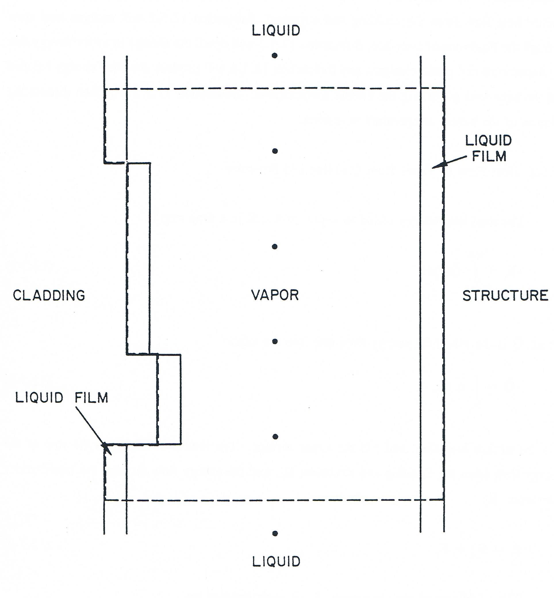
Figure 12.5.1 Control volume for the Uniform Vapor Pressure Model (control volume is outlines by the dashed line)

12.5.1. Heat Flow to Vapor from Cladding and Structure

The total heat energy added to vapor bubble $K$ in a time step is

(12.5-1) $$E_{t} = \int_{t}^{t + \Delta t}{\widetilde{Q}\left( \tau \right)d\tau}$$

where $\widetilde{Q}$ is the total heat energy flow rate into the vapor:

(12.5-2) $$\widetilde{Q} = \int_{s}^{}q ds$$

$q$ is the surface heat flux, and $s$ is the vapor surface. The total heat energy is the sum of the energy flow from the cladding and structure, $E_{es}$, and the energy flow through the liquid-vapor interfaces, $E_{i}$:

(12.5-3) $$E_{t} = E_{es} + E_{i}$$

The cladding and structure term, $E_{es}$ is approximated by

(12.5-4) $$E_{es} = \frac{\Delta t}{2}\left\lbrack Q_{es}\left( K,t \right) + Q_{es}(K,t + \Delta t) \right\rbrack$$

where $Q_{es}$ is the heat flow from the cladding and structure,

(12.5-5) $$Q_{es}\left( K,t \right) = P_{e}\int_{z_{i}(L = 1,t,K)}^{z_{2}(L = 2,t,K)}{\lbrack q_{e}\left( z,t \right) + \gamma_{2}q_{s}(z,t)\rbrack}dz$$

with

$z_{i}\left(2, t, K \right) =$ height of upper liquid-vapor interface

$z_{i}\left(1, t, K \right) =$ height of lower liquid-vapor interface

$P_{e} =$ perimeter of cladding $= 2\pi r_{e}$

$r_{e} =$ nominal radius of cladding

$\gamma_{2} =$ ratio of surface area of structure to surface area of cladding

$q_{e} =$ cladding-to-vapor heat flux

and

$q_{s} =$ structure-to-vapor heat flux.

The heat fluxes are calculated from Newton’s law of cooling as

(12.5-6) $$q_{e}\left( z,t \right) = \frac{T_{e}\left( z,t \right) - T(K,t)}{R_{ec}(z,t)}$$

and

(12.5-7) $$q_{s}\left( z,t \right) = \frac{T_{s}\left( z,t \right) - T(K,t)}{R_{sc}(z,t)}$$

where $T \left(K, t \right)$ is the uniform temperatures within bubble $K$ at time t and $R_{ec}$ and $R_{sc}$ are the thermal resistances between the cladding and vapor and he structure and vapor, respectively.

The form of the thermal resistances is best discussed in terms of a thermal network. Focusing first on the cladding-vapor resistance, Figure 12.5.2 shows the thermal network formed by the cladding, liquid film on the cladding, and vapor and gives the thermal resistances associated with each region. Because of the high thermal conductivity of liquid metals, the resistance of the liquid sodium film can be taken to be just the conductive resistance. The total thermal resistance is then the sum of the individual resistances, or

(12.5-8) $$R_{ec} = \frac{1}{h_{ec}} + R_{ehf}$$

where $R_{ehf}$ is the resistance of the cladding, as discussed in Chapter 3 (see Section 3.5.1, Eq. (3.5-7)) and $h_{ec}$ is the heat-transfer coefficient which models the combined resistances of the liquid film and the vapor. The coefficient $h_{ec} \text{ is just } \frac{1}{\frac{1}{h_{c}} + \frac{w_{fe}}{k_{l}}}$; however, this is not as simple an expression as it appears, since the convective heat-transfer coefficient $h_{c}$ is not a constant or a simple function of temperature. To circumvent this difficulty, a temperature correlation based on physical data was developed for $h_{ec}$ and used in SASSYS-1. This correlation is based on the temperature difference between the cladding and the vapor and is structured as follows. If the cladding is more than 100 K hotter than the vapor, the liquid film is assumed to be at the same temperature as the vapor, which amounts to neglecting the thermal resistance of the vapor. The coefficient $h_{ec}$ then takes the form

(12.5-9) $$h_{ec}\left( z \right) = \frac{k_{l}(z)}{w_{fe}(z)}\ \text{if }T_{e}\left( z \right) > T\left( K \right) + 100$$

where

$k_{l} \left( z \right) =$ thermal conductivity of liquid sodium at temperature $T \left( K \right)$

and

$w_{fe} \left( z \right) =$ thickness of liquid film on the cladding

and $T \left( K \right)$ represents an extrapolated vapor temperature for advanced time values of $h_{ec}$. If the cladding is more than 100 K colder than the vapor, the liquid film is assumed to be at the same temperature as the cladding, and so the resistance of the film is neglected. The heat-transfer coefficient from the vapor to the film is a condensation coefficient $h_{cond}$ which is supplied by the user through the input variable HCOND. A reasonable value for HCOND is around $6\times10^{4} \text{ W/m}^{2}\text{ K}$. The coefficient $h_{ec}$ then becomes

(12.5-10) $$h_{ec}\left( z \right) = h_{cond}\ \text{if }T_{e}\left( z \right) < T\left( K \right) - 100$$

For $T\left( K \right) - 100 \leq T_{e}\left( z \right) \leq T\left(K\right) + 100 \text{,} h_{ec}$ is calculated as an interpolation of the condensation coefficient and the conductive film resistance according to the formula

(12.5-11) $$h_{ec}\left( z \right) = h_{cond} + \frac{\frac{k_{l}\left( z \right)}{w_{fe}(z)} - h_{cond}}{1 + \exp\left\lbrack \frac{T\left( K \right) - T_{e}\left( z \right)}{2} \right\rbrack}\ ,T\left( K \right) - 100 \leq T_{e}\left( z \right) \leq T\left( K \right) + 100$$

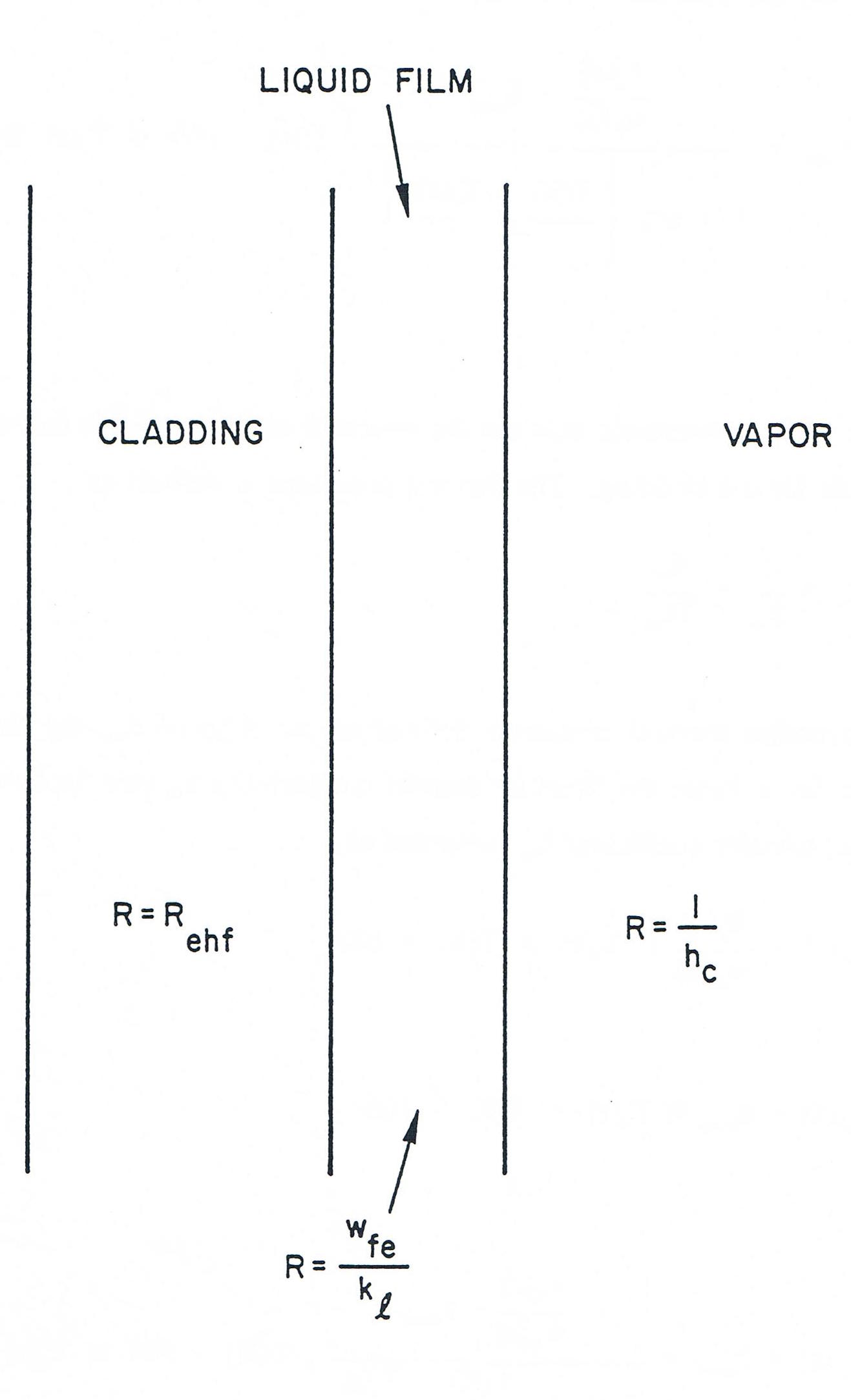
Figure 12.5.2 Thermal Network Formed by the Cladding, Cladding Film, and Vapor

The thermal resistance between the structure and he vapor is calculated using the same procedure as for the cladding. The thermal resistance is defined as

(12.5-12) $$R_{sc} = \frac{1}{h_{sc}} + \frac{d_{sti}}{2k_{sti}}$$

with the structure thermal resistance defined as the ratio of $d_{sti}$, the thickness of the inner structure node, to twice the structure thermal conductivity $k_{sti}$ (see Section 3.5.2, Eq. (3.5-18)), and the heat-transfer coefficient $h_{sc}$ computed as

(12.5-13) $$h_{sc}\left( z \right) = \frac{k_{l}(z)}{w_{fs}(z)}\ \text{ if }T_{s}\left( z \right) > T\left( K \right) - 100$$

(12.5-14) $$h_{sc}\left( z \right) = h_{cond}\ \text{ if }T_{s}\left( z \right) < T\left( K \right) - 100$$

and

(12.5-15) $$h_{sc}\left( z \right) = h_{cond} + \frac{\frac{k_{l}(z)}{w_{fe}(z)} - h_{cond}}{1 + \text{exp}\left\lbrack \frac{T\left( K \right) - T_{e}(z)}{2} \right\rbrack}\ ,T\left( K \right) - 100 \leq T_{s}\left( z \right) \leq T\left( K \right) + 100$$

where $w_{fs}\left( z \right)$ is the thickness of liquid film on the structure.

With the cladding-to-vapor and structure-to-vapor heat fluxes now defined, Eq. (12.5-5) can be solved for $Q_{es}\left(K, t \right)$ in terms of known quantities. The problem how is to use Eq. (12.5-5) to express $Q_{es}\left(K, t + \Delta t \right)$ as a linear function of the change in vapor temperatures over the time step $\Delta t$. The difficulty comes from the fact that the advanced time interface positions $z_{i}$ (which are the limits of integration in the expression for $Q_{es}\left(K, t + \Delta t \right)$ are dependent on the advanced time vapor pressures and, therefore, on the advanced time temperatures. However, $Q_{es}\left(K, t + \Delta t \right)$ can be written as a linear function of the temperature changes if the interface positions are written as the sum of two functions, one which contains only known quantities and one which is a linear function of the change in vapor temperature. To this end, the interface position at $\left(t + \Delta t \right)$ can be written as a linear function

(12.5-16) $$z_{i}\left( L,t + \Delta t,K \right) = z_{i}\left( L,t,K \right) + \Delta z_{i}(K,L)$$

with the change in position $\Delta z_{i}$ given by

(12.5-17) $$\Delta z_{i}\left( K,L \right) = \frac{\Delta t}{2}(v_{i}\left( L,t,K \right) + v_{i}\left( L,t + \Delta t,K \right))$$

The advanced time interface velocity can also be expressed as a linear function

(12.5-18) $$v_{i}\left( L,t + \Delta t,K \right) = v_{i}\left( L,t,K \right) + \Delta v_{i}(K,L)$$

with the change in interface velocity computed from the change in liquid slug mass flow rate

(12.5-19) $$\Delta v_{i}\left( K,L \right) = \frac{\Delta W(K')}{\left( \rho_{l}A_{c} \right)_{K',L}}$$

where

(12.5-20) $$K' = K\text{ if }L = 1$$

(12.5-21) $$K' = K + 1\ \text{ if }L = 2$$

and $\left( \rho_{l}A_{c} \right)_{K', L}$ is the product of the liquid density and channel flow area at the bubble interface. It is assumed in Eq. (12.5-19) that the change in interface velocity can be expressed as the change in the average slug velocity (see Eq. (12.3-1)), with the correction for film thickness ignored. If now the expression for the change in liquid slug mass flow rate, Eq. (12.2-38) derived in Section 3.2, is combined with Eq. (12.5-19) and inserted into Eq. (12.5-8), the advanced time interface velocity becomes

(12.5-22) $$v_{i}\left( L,t + \Delta t,K \right) = v_{i}\left( L,t,K \right) + \frac{1}{(\rho_{l}A_{c})_{K',L}} \frac{\Delta t\lbrack AA_{0}\left( K' \right) + \left( \Delta p_{K' - 1} - \Delta p_{K'} \right)\theta_{2}\rbrack}{I_{1}\left( K' \right) + \theta_{2}\Delta I_{1}\left( K' \right) + \theta_{2}BB_{0}\left( K' \right)\Delta t}$$

where $\Delta p_{K}$ is the change in pressure in bubble $K$ during the time step and $K'$ is defined as above. Substituting Eq. (12.5-17) and Eq. (12.5-22) into Eq. (12.5-16) gives the advanced time interface position as

(12.5-23) $$z_{i}\left( L,t + \Delta t,K \right) = z_{i}\left( L,t,K \right) + v_{i}\left( L,t,K \right)\Delta t + \frac{\Delta t}{2}\frac{1}{{{(\rho}_{l}A_{c})}_{K',L}}\frac{\Delta t\lbrack AA_{0}\left( K' \right) + \left( \Delta p_{K' - 1} - \Delta p_{K'} \right)\theta_{2}\rbrack}{I_{1}\left( K' \right) + \theta_{2}\Delta I_{1}\left( K' \right) + \theta_{2}BB_{0}\left( L' \right)\Delta t}$$

which can be rewritten as

(12.5-24) $$z_{i}\left( L,t + \Delta t,K \right) = z_{i0}\left( K,L \right) + \Delta z'(K,L)$$

where $z_{i0}\left( K,L \right)$ is the function

(12.5-25) $$z_{i0}\left( K,L \right) = z_{i}\left( L,t,K \right) + \Delta z_{0}(K,L)$$

with

(12.5-26) $$\Delta z_{i0}\left( K,L \right) = v_{i}\left( L,t,K \right) + \frac{1}{2}\frac{\Delta W_{0}\left( K' \right)\Delta t}{{(\rho_{l}A_{c})}_{K',L}}$$

and

(12.5-27) $$\Delta W_{0}\left( K' \right) = \frac{AA_{0}\left( K' \right)\Delta t}{I_{1}\left( K' \right) + \theta_{2}\Delta I_{1}\left( K' \right) + BB_{0}\left( K' \right)\theta_{2}\Delta t}$$

and $\Delta z'\left( K,L \right)$ is

(12.5-28) $$\Delta z'\left( K,L \right) = \frac{dz_{i}\left( K,L \right)}{dp}(\Delta p_{K' - 1} - \Delta p_{K'})$$

with

(12.5-29) $$\frac{dz_{i}(K,L)}{dp} = \frac{\theta_{2}\Delta t^{2}}{2{(\rho_{l}A_{c})}_{K',L}\lbrack I_{1}\left( K' \right) + \theta_{2}\Delta I_{1}\left( K' \right) + BB_{0}\left( K' \right)\theta_{2}\Delta t\rbrack}$$

The expression for $\frac{dz_{i}}{dp}$ is obtained by taking the derivative with respect to pressure of Eq. (12.5-17), using Eq. (12.5-22). The function $z_{i0}$ is a function only of known quantities and is the approximate position to which the interface would move at $t + \Delta t$ if the bubble pressures did not change over the time step. The additional change in interface position due to bubble pressure changes is accounted for by $\Delta z'$, which is a linear function of the pressure changes.

Using Eq. (12.5-24) for the interface position, the integral for the cladding and structure heat flow $Q_{es}\left(K, t + \Delta t \right)$ can be expressed as the sum of three integrals:

(12.5-30) $$\begin{split}Q_{es}\left( K,t + \Delta t \right) = P_{e}\int_{{z_{i}}_{0}\left( K,1 \right)}^{{z_{i}}_{0}\left( K,2 \right)}{\left\lbrack q_{e}\left( z,t + \Delta t \right) + \gamma_{2}q_{s}\left( z,t\Delta t \right) \right\rbrack dz} \\ + P_{e}\int_{{z_{i}}_{0}\left( K,2 \right)}^{{z_{i}}_{0}\left( K,2 \right) + \Delta z'\left( K,1 \right)}{\left\lbrack q_{e}\left( z,t + \Delta t \right) + \gamma_{2}q_{s}\left( z,t\Delta t \right) \right\rbrack dz} \\ + P_{e}\int_{{z_{i}}_{0}\left( K,1 \right) + \Delta z'\left( K,1 \right)}^{{z_{i}}_{0}\left( K,1 \right)}{\left\lbrack q_{e}\left( z,t + \Delta t \right) + \gamma_{2}q_{s}(z,t\Delta t) \right\rbrack dz}\end{split}$$

If the vapor temperature $T \left(K, t + \Delta t \right)$ is linearized to be $T\left(K,t \right) + \Delta T \left( K \right)$, the first integral is a function only of $\Delta T \left( K \right)$ and known quantities, since the advanced time cladding and structure temperatures are determined by extrapolation from values calculated in the transient heat-transfer module at the previous two heat-transfer time steps and, therefore, are considered known. Using Eq. (3.5-6) for the heat fluxes, the first integral can be written as the sum $I_{e1} \left( K \right) + I_{e2} \left( K \right) \Delta T \left( K \right)$, where

(12.5-31) $$\begin{split}I_{e1}\left( K \right) = P_{e}\int_{{z_{i}}_{0}(K,1)}^{{z_{i}}_{0}(K,2)}\bigg\{ \frac{T_{e}\left( z,t + \Delta t \right) - T\left( K,t \right)}{R_{ec}\left( z,t + \Delta t \right)} \\ + \frac{\gamma_{2}\lbrack T_{s}\left( z,t + \Delta t \right) - T(K,t)\rbrack}{R_{sc}(z,t + \Delta t)} \bigg\}dz\end{split}$$

and

(12.5-32) $$I_{e2}\left( K \right) = - P_{e}\int_{{z_{i}}_{0}(K,1)}^{{z_{i}}_{0}(K,2)}{\left\lbrack \frac{1}{R_{ec}\left( z,t + \Delta t \right)} + \frac{\gamma_{2}}{R_{sc}(z,t + \Delta t} \right\rbrack dz}$$

The second and third integrals are evaluated by assuming that the heat fluxes are constant in space over the domain of integration; this is a reasonable assumption, since $\Delta z$ is a small quantity. If second-order terms proportional to $\Delta T \Delta z'$ are dropped, the second integral is just $I_{e3}\left(K \right) \Delta z' \left(K, 2\right)$, with

(12.5-33) $$\begin{split}I_{e3}\left( K \right) = P_{e}\bigg\{ \frac{T_{e}\left\lbrack {z_{i}}_{0}\left( K,2 \right),t + \Delta t \right\rbrack - T\left( K,t \right)}{R_{ec}\left\lbrack {z_{i}}_{0}\left( K,2 \right),t + \Delta t \right\rbrack} \\ + \gamma_{2}\left\lbrack \frac{T_{s}\left\lbrack z_{i_{0}}\left( K,2 \right),t + \Delta t \right\rbrack - T(K,t)}{R_{sc}\lbrack{z_{i}}_{0}\left( K,2 \right),t + \Delta t\rbrack} \right\rbrack \bigg\}\end{split}$$

and the third integral is $I_{e3}\left(K \right) \Delta z' \left(K, 1\right)$, where

(12.5-34) $$\begin{split}I_{e4}\left( K \right) = - P_{e}\Bigg\{ \frac{T_{e}\left\lbrack {z_{i}}_{0}\left( K,1 \right),t + \Delta t \right\rbrack - T(K,t)}{R_{ec}\lbrack{z_{i}}_{0}\left( K,1 \right),t + \Delta t\rbrack} \\ + \gamma_{2}\left\lbrack \frac{T_{s}\left\lbrack z_{i_{0}}\left( K,1 \right),t + \Delta t \right\rbrack - T(K,t)}{R_{sc}\lbrack z_{i_{0}}\left( K,1 \right),t + \Delta t\rbrack} \right\rbrack \Bigg\}\end{split}$$

This gives for $Q_{es}\left( K,t + \Delta t \right)$

(12.5-35) $$Q_{es}\left( K,t + \Delta t \right) = I_{e1}\left( K \right) + I_{e2}\left( K \right)\Delta T\left( K \right) + I_{e3}\left( K \right)\Delta z'\left( K,2 \right) + I_{e4}\left( K \right)\Delta z'(K,1)$$

which, by the definition of $\Delta z'$ and the assumption of saturation conditions, is a function only of known quantities and the changes in bubble temperatures.

Note that Eq. (12.5-35) is valid regardless of the direction of motion of either interface. The sign of $\Delta z'$ will be positive for upward interface motion and negative for downward motion, giving the correct sign to the last two terms in Eq. (12.5-35).

The energy flow in $E_{es}$ is therefore given by the linear equation

(12.5-36) $$\begin{split}E_{es} = \frac{\Delta t}{2}\bigg[ Q_{es}\left( K,t \right) + I_{e1}\left( K \right) + \bigg( I_{e2}\left( K \right) + I_{e3}\left( K \right)\frac{dz_{i}\left( K,2 \right)}{dp} \\ - I_{e4}\left( K \right)\frac{dz_{i}\left( K,1 \right)}{dp} \bigg)\Delta p_{K} - I_{e3}\left( K \right)\frac{dz_{i}\left( K,1 \right)}{dp}\Delta p_{K + 1} \\ + I_{e4}\left( K \right)\frac{dz_{i}\left( K,1 \right)}{dp}\Delta p_{K - 1}\bigg]\end{split}$$

where the definition of $\Delta z^{i}$ in terms of $\Delta p$ has been used.

12.5.2. Heat Flow through Liquid-Vapor Interface

The SASSYS-1 calculation of the heat flow through the liquid-vapor interface is based on the work by Cronenberg [12-7]. In the method, the total heat flow through the liquid-vapor interfaces is the sum of an upper interface term $I_{iu}$ and a lower interface term $I_{il}$

(12.5-37) $$E_{i} = \Delta t(I_{iu} + I_{il})$$

where

(12.5-38) $$I_{ix} = k_{l}A_{cx}{\frac{\overline{\partial{T_{l}}_{x}}}{\partial\xi}\bigg|}_{\xi = 0}$$

with

$x = u \text{ or } l$

$A_{cx} =$ area of coolant channel

$T_{l x} =$ liquid temperature near interface

$k_{l} =$ liquid thermal conductivity near interface

$\xi =$ axial distance from interface

$\xi =z - z_{i}$ for upper interface

$\xi = -\left(z - z_{i} \right)$ for lower interface

and

$\frac{\overline{\partial{T_{l}}_{x}}}{\partial\xi}$ is the time average of the spatial derivative for the time step

An expression for the coolant temperature derivative $\frac{\overline{\partial{T_{l}}_{x}}}{\partial\xi}\ $can be derived from the general heat conduction equation written for the liquid slug as

(12.5-39) $$\alpha\frac{\partial^{2}T_{l}(\xi,t')}{\partial\xi^{2}} + \frac{Q(\xi,t')}{\rho_{l}C_{l}} = \frac{\partial^{2}T_{l}\left( \xi,t' \right)}{\partial t'}$$

where

$\alpha = k_{l} / \rho_{l}C_{l}$, the thermal diffusivity of liquid sodium

$k_{l} =$ thermal conductivity of the liquid

$C_{l} =$ liquid heat capacity

$\rho_{l} =$ liquid density

$Q =$ heat input per unit volume in the liquid

$T_{l} =$ temperature in liquid slug

$\xi =$ distance into liquid slug form liquid-vapor interface

and

$t' =$ time since the vapor bubble started to form

The heat input $Q$ includes both the direct heating $Q_{c}$ and the heat flow $Q_{ec} + Q_{sc}$ from the cladding and structure to the liquid slug:

(12.5-40) $$Q = Q_{c} + Q_{ec} + Q_{sc}$$

where the functional form of $Q_{c}$ is given in Chapter 3, Eq. (3.3-6), and $Q_{ec} \text{ and } Q_{sc}$ are calculated form Newton’s law of cooling in the form of Eq. (3.3-7) and Eq. (3.3-8) in Chapter 3.

The boundary conditions for the problem are

(12.5-41) $$T_{l}\left( \xi = 0,t' \right) = T\left( t' \right) \text{, the vapor temperature at the liquid-vapor interface}$$

and

(12.5-42) $$T_{l}\left( \xi = \infty,t' \right) < \infty$$

and the initial condition is

(12.5-43) $$T_{l}(\xi,t' = 0)$$

The heat conduction equation, together with the initial and boundary conditions, can be solved for $T_{l}$ through the use of the Laplace transform method. The details of this approach are presented in Section 12.16; here, just the main points will be listed. The procedure involves four main stages:

1. Take the Laplace transform of the heat conduction equation, Eq. (12.5-39). This produces a second-order ordinary differential equation in space.

2. Solve the differential equation produced in stage 1 for the Laplace transform of $T_{l}$ as a function of $\xi$.

3. Take the spatial derivative of the Laplace transform of $T_{l}$ and evaluate it at $\xi = 0$.

4. Take the inverse Laplace transform of the derivative from stage 3, producing ${\frac{\partial T_{l}}{\partial\xi}\Big|}_{\xi = 0}$

This procedure results in the following expression for ${\frac{\partial T_{l}}{\partial\xi}\Big|}_{\xi = 0}$

(12.5-44) $$\begin{split}\frac{\partial T_{l}\left( \xi = 0,t' \right)}{\partial\xi} = \frac{- 1}{\sqrt{\pi \alpha}}\int_{0}^{t'}\frac{\partial T_{l}\left( \xi = 0,\tau \right)}{\partial\tau}\frac{1}{\sqrt{t' - \tau}}d\tau \\ - \frac{T_{l} \left( \xi = 0, t' = 0 \right)}{\sqrt{\alpha \pi t'}} + \int_{0}^{\infty} d\xi \int_{0}^{t'} \frac{\xi Q \left(\xi, \tau \right) \text{exp} \left[-\frac{\xi^{2}}{4 \alpha \left(t' - \tau \right)} \right]}{2k_{l} \sqrt{\pi \alpha \left(t' - \tau \right)^{3}}} d\tau \\ + \int_{0}^{\infty} \frac{T_{l} \left(\xi, t' = 0 \right) \xi \text{ exp} \left[ -\frac{\xi^{2}}{4 \alpha t'} \right]}{2 \alpha \sqrt{\pi \alpha \left( t' \right)^{3}}} d\xi\end{split}$$

To evaluate the terms in Eq. (12.5-44), first note that the exponential function in the third and fourth terms decays very rapidly with increasing $\xi$ due to the small thermal diffusivity of liquid sodium. Therefore, for purposes of solving Eq. (12.5-44), it is valid to assume that the initial temperature distribution $\left( t' = 0 \right)$ is uniform near the interface, or

(12.5-45) $$T_{l}\left( \xi,t' = 0 \right) = T_{0}$$

Then the fourth term in Eq. (12.5-44) is easily integrated to give

(12.5-46) $$\int_{0}^{\infty}\frac{T_{0}}{\alpha}\frac{\xi exp\lbrack - \xi^{2}/4\alpha t'\rbrack}{2\sqrt{\pi\alpha \left( t' \right)^{3}}}d\xi = \frac{T_{0}} {\sqrt{\pi \alpha t'}}$$

so the second and fourth terms cancel.

Similarly, $Q \left(\xi , \tau \right)$ can be approximated as the spatially constant function $Q_{Ox} \left(\tau \right)$ near the interface so the third term becomes

(12.5-47) $$\int_{0}^{t'}d\tau\int_{0}^{\infty}d\xi\frac{\xi Q_{Ox}\exp\left\lbrack - \frac{\xi^{2}}{4\alpha\left( t' - \tau \right)} \right\rbrack}{2k_{l}\sqrt{\pi \alpha\left( t' - \tau \right)^{3}}} = \int_{0}^{t'}\frac{d\tau Q_{Ox}\left( \tau \right)}{k_{l}}\left( \frac{\alpha}{\pi(t' - \tau} \right)^{1/2}$$

with $Q_{Ox}\left( \tau \right)$ defined as

(12.5-48) $$Q_{Ox}\left( \tau \right) = \gamma \left[\frac{T_{e_{x}} \left( \tau \right) - T\left( \tau \right)}{R_{ecx}} + \gamma_{2}\frac{T_{s_{x}}\left( \tau \right) - T(\tau)}{R_{scx}}\ \right]$$

where

$\gamma =$ ratio of cladding surface area to coolant volume

$\gamma_{2} =$ ratio of surface area of structure to surface area of cladding

$R_{ecx} =$ thermal resistance between the cladding and the coolant at the interface

$R_{scx} =$ thermal resistance between the structure and the coolant at the interface

and

$$\begin{split}x = \bigg\{\begin{matrix} \text{U at the upper interface} \\ l \text{ at the lower interface} \\ \end{matrix}\end{split}$$

Thus, Eq. (12.5-44) has the reduced form

(12.5-49) $$\frac{\partial T_{1}}{\partial\xi}\left( \xi = 0,t' \right) = \frac{1}{\sqrt{\pi}}\int_{0}^{t'}{\left[ Q_{Ox}\left( \tau \right)\frac{\sqrt{a}}{k_{l}} - \frac{1}{\sqrt{a}}\frac{\partial T_{l}}{\partial\tau}(\xi = 0,\tau)\ \right]}\ \frac{d\tau}{\sqrt{t' - r}}$$

which can be rewritten in terms of t, the time since initiation of the transient, through the variable transformation $t' = t - t_{b}$:

(12.5-50) $$\left. \ \frac{\partial{T_{l}}_{x}(t)}{\partial\xi} \right|_{\xi = 0} = \frac{1}{\sqrt{\pi}}\int_{t_{b}}^{t}{\left\lbrack Q_{\text{Ox}}\left( \tau \right)\frac{\sqrt{a}}{k_{l}} - \frac{1}{\sqrt{a}}\frac{\partial T\left( \tau \right)}{\partial\tau}\ \right\rbrack\frac{d\tau}{\sqrt{t - r}}}$$

The boundary condition at $\xi = 0$ has been incorporated into this expression. Eq. (12.5-50) will be somewhat easier to work with if the function

(12.5-51) $$f_{x}\left( \tau \right) \equiv Q_{\text{Ox}}\left( \tau \right)\frac{\sqrt{a}}{k_{l}} - \frac{1}{\sqrt{a}}\frac{\partial T\left( \tau \right)}{\partial\tau}$$

is used to give the simpler equation

(12.5-52) $$\left. \ \frac{\partial{T_{l}}_{x}(t)}{\partial\xi} \right|_{\xi = 0} = \frac{1}{\sqrt{\pi}}\int_{t_{b}}^{t}{\frac{d\tau}{\sqrt{t - \tau}}f_{x}(\tau)}$$

Now, the time average over the time step $\Delta t$ of $\left. \ \frac{\partial{T_{l}}_{x}(t)}{\partial\xi} \right|_{\xi = 0}$needed to compute the interface heat flow from Eq. (12.5-60) can be written as

(12.5-53) $$\frac{\partial \overline{T}_{l_{x}}}{\partial \xi} \bigg|_{\xi = 0 } = \frac{1}{\Delta t}\int_{0}^{\Delta t}d\varepsilon \frac{\partial{T_{l}}_{x}(t_{k} + \varepsilon)}{\partial\xi} \bigg|_{\xi = 0}$$

with $\left. \ \frac{\partial{T_{l}}_{x}(t)}{\partial\xi} \right|_{\xi = 0}$expressed as in Eq. (12.5-52) and $t = t_k$ the time at the beginning of the time step. To accomplish the goal of expressing the energy balance for the bubble as a linear function of the vapor temperatures, the integral in Eq. (12.5-53) must be written as a linear function of the vapor temperatures. This in turn means that the function $f_{x}\left( \tau \right)$ must be approximated so that Eq. (12.5-52) can be integrated and so that the resulting expression is linear in the vapor temperature. This can be done by writing $\left. \ \frac{\partial{T_{l}}_{x}(t)}{\partial\xi} \right|_{\xi = 0}$

(12.5-54) $$\begin{split}\frac{\partial{T_{l}}_{x} (t + \varepsilon)}{\partial\xi} |_{\xi = 0} = \frac{1}{\sqrt{\pi}} \int_{t_{b}}^{t_{k} + \varepsilon} \frac{d\tau}{\sqrt{t_{k} - \tau + \varepsilon}} f_{x} \left(\tau \right) \\ = \frac{1}{\sqrt{\pi}}\int_{t_{b}}^{t_{k}}\frac{d\tau}{\sqrt{t_{k} - \tau + \varepsilon}}f_{x}\left( \tau \right) + \frac{1}{\sqrt{\pi}}\int_{t_k}^{t_{k} + \varepsilon}\frac{d\tau}{\sqrt{t_{k} - \tau + \varepsilon}} f_{x} \left(\tau \right)\end{split}$$

The first term in Eq. (12.5-54) is a function only of known quantities, since the range of integration extends only up to the beginning of the current time step. Therefore, the dependence on advanced time vapor temperatures is contained entirely in the second term of Eq. (12.5-54). To integrate this term, define the quantity $\overline{f}_{x \Delta t}$ to be the simple average of $f_x(\tau)$ over the range of integration:

(12.5-55) $$\begin{align}\begin{aligned}{\overline{f}}_{x\Delta t} &= \frac{1}{\Delta t}\int_{t_{k}}^{t_{k} + \Delta t}{dt f_{x}\left( t \right)}\\&= \frac{1}{\Delta t}\int_{t_{k}}^{t_{k} + \Delta t}{dt\left\lbrack Q_{\text{Ox}}\left( t \right)\frac{\sqrt{a}}{k_{l}} - \frac{1}{\sqrt{a}}\frac{\partial T(t)}{\partial t} \right\rbrack}\end{aligned}\end{align}$$

If the cladding, structure, and vapor temperatures in the expression given above for $Q_{Ox}$ are assumed linear in time over $\Delta t$, ${\overline{f}}_{x\Delta t}$becomes

(12.5-56) $$\begin{align}\begin{aligned}{\overline{f}}_{x\Delta t} &= \frac{1}{\Delta t}\left\lbrack \frac{\sqrt{\alpha}}{k_{l}}\frac{\Delta t}{2}\left( Q_{\text{Ox}}\left( t_{k} \right) + Q_{\text{Ox}}\left( t_{k} + \Delta t \right) \right) - \frac{1}{\sqrt{\alpha}}(T\left( t_{k} + \Delta t \right) - T(t_{k}))\ \right\rbrack\\& = \frac{1}{2}\left\lbrack Q_{\text{Ox}}\left( t_{k} \right) + Q_{\text{Ox}}\left( t_{k} + \Delta t \right) \right\rbrack\frac{\sqrt{\alpha}}{k_{l}} - \frac{1}{\sqrt{\alpha}}\frac{T\left( t_{k} + \Delta t \right) - T\left( t_{k} \right)}{\Delta t}\end{aligned}\end{align}$$

Since $\Delta t$ (and therefore $\varepsilon$) is small, it is reasonable to approximate $f_{x}\left(t \right)$ as ${\overline{f}}_{x\Delta t}$ from $t_{k}$ to $t_{k} + \varepsilon$. Thus, the second term in Eq. (12.5-54) becomes

(12.5-57) $$\frac{1}{\sqrt{\pi}}\int_{t_{k}}^{t_{k} + \varepsilon}{\frac{d\tau}{\sqrt{t_{k} - \tau + \varepsilon}}f_{x}\left( \tau \right) = \frac{1}{\sqrt{\pi}}\int_{t_{k}}^{t_{k} + \varepsilon}{\frac{d\tau}{\sqrt{t_{k} - \tau + \varepsilon}}{\overline{f}}_{x\Delta t}}}$$

This equation can be integrated easily by making the change of variable $\tau ' = t_{k} - \tau + \varepsilon$ to give

(12.5-58) $$\frac{1}{\sqrt{\pi}}\int_{t_{k}}^{t_{k} + \varepsilon}\frac{d\tau}{\sqrt{t_{k} - \tau + \varepsilon}}{\overline{f}}_{x\Delta t} = {\overline{f}}_{x\Delta t}\int_{0}^{\epsilon}{\frac{d\tau'}{\sqrt{\tau'}} = 2\sqrt{\varepsilon}}{\overline{f}}_{x\Delta t}$$

which is linear in $T \left(T_{k} + \Delta t \right)$.

The interface heat flow has now been expressed as a linear function of the advanced time vapor temperature. However, one problem remains; namely, evaluation of the integral in the first term in Eq. (3.5-47). One simple way to handle this is to approximate $f_x \left( \tau \right)$ by some average value $\overline{f}_x$ over the range of integration, giving

(12.5-59) $$\begin{align}\begin{aligned}\begin{split}\int_{t_{b}}^{t_{k}}\frac{d\tau}{\sqrt{t_{k} + \varepsilon - \tau}}f_{x}\left( \tau \right) &= {\overline{f}}_{x}\int_{t_{b}}^{t_{k}}\frac{d\tau'}{\sqrt{\tau_{k} - \varepsilon - \tau}}\\\end{split}\\&= {\overline{f}}_{x}\int_{\varepsilon}^{t_{k} + \varepsilon - t_{b}}\frac{d\tau'}{\sqrt{\tau'}}\\&= 2{\overline{f}}_{x}(\sqrt{\tau_{k} + \varepsilon - \tau_{b}} - \sqrt{\varepsilon})\end{aligned}\end{align}$$

where the integral has been evaluated using the change of variable $\tau ' = t_{k} + \varepsilon - \tau$ as above. Now, the problem reduces to one of selecting an appropriate value for ${\overline{f}}_{x}$. The range of integration is too large to use the simple average as was done above. An alternative approach, is to examine the integral in the first term of Eq. (12.5-54) and try to develop an expression for $\overline{f}_x$ which is a function of $t_{k}$ and which can be computed form values at earlier time steps through a recursion relation. To this end, use the fact that $\varepsilon$ is small to approximate the first integral in Eq. (12.5-54) as

(12.5-60) $$\begin{align}\begin{aligned}\int_{t_{b}}^{t_{k}}\frac{d\tau}{\sqrt{t_{k} + \varepsilon - \tau}}f_{x}(\tau) &\approx \int_{t_{b}}^{t_{k}}{\frac{d\tau}{\sqrt{t_{k} - \tau}}f_{x}(\tau)}\\&= \int_{0}^{t_{k} - t_{b}}\frac{d\tau'}{\sqrt{\tau'}}f_{x}(t_{k} - \tau')\end{aligned}\end{align}$$

The transformation $\tau ' = t_{k} - \tau$ was used in the last integral in Eq. (12.5-60). Now, define the function $g_{x}\left( \tau ' \right)$ as

(12.5-61) $$g_{x}\left( \tau' \right) = f_{x}(t_{k} - \tau')$$

and the weighted average of $g_{x}$ as

(12.5-62) $${\overline{g}}_{x}\left( t_{k} \right) = \frac{\int_{0}^{t_{k} - t_{b}}\frac{d\tau'}{\sqrt{\tau'}}g_{x}\left( \tau' \right)}{\int_{0}^{t_{k} - t_{b}}\frac{d\tau'}{\sqrt{\tau'}}}$$

As will be shown below, ${\overline{g}}_{x}(t_{k})$can be determined form a recursion relation.

Rearranging Eq. (12.5-62) gives the integral in Eq. (12.5-60) the form

(12.5-63) $$\int_{0}^{t_{k} - t_{b}}\frac{d\tau'}{\sqrt{\tau'}}f_{x}\left( t_{k} - \tau' \right) = 2\sqrt{\tau_{k} - t_{b}}\,\overline{g}_{x}\left( t_{k} \right)$$

The function ${\overline{f}}_{x}$can now be expressed in terms of ${\overline{g}}_{x}(t_{k})$by combining Eq. (12.5-59), Eq. (12.5-60), and Eq. (12.5-63) to give

(12.5-64) $$\begin{align}\begin{aligned}2{\overline{f}}_{x}\left( \sqrt{t_{k} + \varepsilon - \tau_{b}} - \sqrt{\varepsilon} \right) &= \int_{t_{b}}^{t_{k}}{\frac{d\tau}{\sqrt{t_{k} + \varepsilon - \tau}}f_{x}\left( \tau \right)}\\&\approx \int_{t_{b}}^{t_{k}}{\frac{d\tau}{\sqrt{t_{k} - \tau}}f_{x}(\tau)}\\&= 2\sqrt{t_{k} - t_{b}}\,\overline{g}_{x}\left( t_{k} \right)\end{aligned}\end{align}$$

Since $\varepsilon$ is small compared to $t_{k} - t_{b}$ for all but the times right after the bubble has formed, it is reasonable to approximate $\sqrt{\tau_{k} + \varepsilon - t_{b}} - \sqrt{\varepsilon}$ $\sqrt{t_{k} - t_{b}}$and therefore to choose

(12.5-65) $${\overline{f}}_{x} = {\overline{g}}_{x}\left( t_{k} \right)$$

as the approximation to $f_{x}(\tau)$ for $t_{b} \leq \tau \leq t_{k}$This expression can be computed from a recursion relation by writing ${\overline{g}}_{x}(t_{k} + \Delta t)$as

(12.5-66) $$\begin{align}\begin{aligned}{\overline{g}}_{x}\left( t_{k} + \Delta t \right) = \int_{0}^{t_{k} + \Delta t - t_{b}}\frac{d\tau'}{\sqrt{\tau'}}f_{x}(t_{k} + \Delta t - \tau')/\int_{0}^{t_{k} + \Delta t - t_{b}}\frac{d\tau'}{\sqrt{\tau'}}\\= \frac{1}{2\sqrt{t_k + \Delta t - t_b}}\left[\int_{0}^{\Delta t}\frac{d\tau'}{\sqrt{\tau'}}f_x(t_k + \Delta t - \tau') + \int_{\Delta t}^{t_k + \Delta t - t_b} \frac{d\tau'}{\sqrt{\tau'}}f_x(t_k + \Delta t - \tau') \right]\end{aligned}\end{align}$$

Substituting the approximations $f_{x}\left( t_{k} + \Delta t - \tau' \right) = {\overline{f}}_{x\Delta t}$ for $0 \leq \tau' \leq \Delta t$ and $f_{x}\left( t_{k} + \Delta t - \tau' \right) = \overline{g}\left( t_{k} \right)$ for $\Delta t \leq \tau' \leq t_{k} + \Delta t - t_{b}$ as used above reduces the integrals in Eq. (12.5-66) to

(12.5-67) $$\begin{align}\begin{aligned}{\overline{g}}_{x}\left( t_{k} + \Delta t \right) &= \frac{1}{2\sqrt{t_{k} + \Delta t - t_{b}}}\left\lbrack \int_{0}^{\Delta t}\frac{d\tau'}{\sqrt{\tau'}}{\overline{f}}_{x\Delta t} + \int_{\Delta t}^{t_{k} + \Delta t - t_{b}}{\frac{d\tau'}{\sqrt{\tau'}}{\overline{g}}_{x}\left( t_{k} \right)} \right\rbrack\\&= \frac{1}{\sqrt{t_{k} + \Delta t - t_{b}}}\left\lbrack {\overline{f}}_{x\Delta t}\sqrt{\Delta t} + {\overline{g}}_{x}\left( t_{k} \right)\left( \sqrt{t_{k} + \Delta t - t_{b}} - \sqrt{\Delta t} \right) \right\rbrack\\&= {\overline{g}}_{x}\left( t_{k} \right)\left\lbrack 1 - \frac{\sqrt{\Delta t}}{\sqrt{t_{k} + \Delta t - t_{b}}} \right\rbrack + {\overline{f}}_{x\Delta t}\frac{\sqrt{\Delta t}}{\sqrt{t_{k} + \Delta t - t_{b}}}\end{aligned}\end{align}$$

so that once the advanced time vapor temperatures are computed, the value of ${\overline{g}}_{x}$for the next time step can be calculated.

With a means now available for obtaining , ${\overline{g}}_{x}(t_{x})$the expression for $\left. \ \frac{\partial{T_{l}}_{x}}{\partial\xi} \right|_{\xi = 0}$in Eq. (12.5-54) can be considered fully determined, and Eq. (12.5-54) can be written

(12.5-68) $$\left. \ \frac{\partial{T_{l}}_{x}(t_{k} + \varepsilon)}{\partial\xi} \right|_{\xi = 0} = \frac{1}{\sqrt{\pi}}\left\lbrack 2{\overline{g}}_{x}\left( t_{k} \right)\left( \sqrt{t_{k} + \varepsilon - t_{b}} - \sqrt{\varepsilon} \right) + 2{\overline{f}}_{x\Delta t}\sqrt{\varepsilon} \right\rbrack$$

The time average of Eq. (12.5-68) is then

(12.5-69) $$\begin{align}\begin{aligned}\left. \ \frac{\overline{\partial{T_{l}}_{x}}}{\partial\xi} \right|_{\xi = 0} &= \frac{2}{\sqrt{\pi}}\frac{1}{\Delta t}\int_{0}^{\Delta t} d\varepsilon \left[{\overline{g}}_{x}\left( t_{k} \right)\left( \sqrt{t_{k} + \varepsilon - t_{b}} - \sqrt{\varepsilon} \right) + {\overline{f}}_{x\Delta t}\sqrt{\varepsilon}\right]\\&= \frac{4}{3\sqrt{\pi}}\frac{1}{\Delta t}\left[{\overline{g}}_{x}\left( t_{k} \right)\left( t_{k} + \Delta t - t_{b} \right)^{\frac{3}{2}} - \left( t_{k} - t_{b} \right)^{\frac{3}{2}} - \left( \Delta t \right)^{\frac{3}{2}} + {\overline{f}}_{x\Delta t}\left( \Delta t \right)^{\frac{3}{2}}\right]\end{aligned}\end{align}$$

Thus, the interface heat flow $I_{ix}$ is, from Eq. (12.5-38) and substituting for ${\overline{f}}_{x\Delta t}$

(12.5-70) $$\begin{split} I_{ix} = k_{l}A_{cx}\frac{4}{3\sqrt{\pi}}\frac{1}{\Delta t}\left\lbrack {\overline{g}}_{x}\left( t \right)\left( \left( t + \Delta t - t_{b} \right)^{\frac{3}{2}} - \left( t - t_{b} \right)^{\frac{3}{2}} - \left( \Delta t \right)^{\frac{3}{2}} \right) \right . \\ \left. + \left( \Delta t \right)^{\frac{3}{2}}\left(\frac{1}{2}\left\lbrack Q_{Ox}\left( t \right) + Q_{Ox}\left( t + \Delta t \right) \right\rbrack\frac{\sqrt{\alpha}}{k_{l}} - \frac{1}{\sqrt{\alpha}}\frac{T\left( t + \Delta t \right) - T(t)}{\Delta t} \right) \right\rbrack\end{split}$$

which, substituting the definition of $Q_{Ox}$, is

(12.5-71) $$\begin{split}I_{ix} = \frac{k_{l}}{\sqrt{\pi}}A_{cx}\frac{4}{3} \Bigg[ {\overline{g}}_{x}\left( t \right)\left( \frac{\left( t + \Delta t - t_{b} \right)^{\frac{3}{2}} - \left( t - t_{b} \right)^{\frac{3}{2}}\ }{\Delta t} - \sqrt{\Delta t} \right) \\ + \sqrt{\Delta t}\Bigg(\frac{\gamma}{2}\left\lbrack \frac{T_{ex}\left( t \right) + T_{ex}\left( t + \Delta t \right) - T\left( t \right) - T\left( t + \Delta t \right)}{R_{ecx}} \right\rbrack \\ + \gamma_{2} \frac{T_{sx}\left( t \right) + T_{sx}\left( t + \Delta t \right) - T\left( t \right) - T\left( t + \Delta t \right)}{R_{scx}} \Bigg] \frac{\sqrt{\alpha}}{k_{l}} \\ - \frac{1}{\sqrt{\alpha}}\frac{T\left( t + \Delta t \right) - T\left( t \right)}{\Delta t} \Bigg]\Bigg) \\ = \frac{4}{3}\frac{k_{l}}{\sqrt{\pi}}A_{cx}{\overline{g}}_{x}\left( t \right)\left( \frac{\left( t + \Delta t - t_{b} \right)^{\frac{3}{2}} - \left( t - t_{b} \right)^{\frac{3}{2}}}{\Delta t} - \sqrt{\Delta t} \right) \\ + \frac{2}{3}\frac{\sqrt{\alpha}}{\sqrt{\pi}}\gamma\sqrt{\Delta t}A_{cx} \Bigg[ \frac{T_{ex}\left( t \right) + T_{ex}\left( t + \Delta t \right) - 2T\left( t \right)}{R_{ecx}} \\ + \gamma_{2}\frac{T_{sx}\left( t \right) + T_{sx}\left( t + \Delta t \right) - 2T\left( t \right)}{R_{scx}} \Bigg] \\ - \Delta T \left[ \frac{2}{3}\frac{\sqrt{\alpha}}{\sqrt{\pi}}A_{cx}\gamma\sqrt{\Delta t}\left( \frac{1}{R_{ecx}} + \frac{\gamma_{2}}{R_{scx}} \right) + \frac{4}{3}\frac{k_{l}}{\sqrt{\pi}}\frac{A_{ex}}{\sqrt{\alpha}}\frac{1}{\sqrt{\Delta t}} \right]\end{split}$$

where $T\left( t + \Delta t \right) = T \left( t \right) + \Delta T$. Using this expression in Eq. (12.5-37) for $E_{i}$, the total heat flow through the liquid-vapor interfaces, gives

(12.5-72) $$E_{i} = \left( I_{i0} + I_{i1}\Delta T \right)\Delta t$$

where

(12.5-73) $$\begin{split}I_{i0} = \frac{k_{l}}{\sqrt{\pi}}\Bigg\{ \sum_{x = u,l}^{}{A_{cx}\Bigg[\frac{2}{3}\frac{\sqrt{\alpha}}{k_{l}}\gamma\sqrt{\Delta t}\Bigg[\frac{T_{ex}\left( t \right) + T_{ex}\left( t + \Delta t \right) - 2T\left( t \right)}{R_{ecx}}} \\ + \gamma_{2}\frac{T_{sx}\left( t \right) + T_{sx}\left( t + \Delta t \right) - 2T\left( t \right)}{R_{scx}} \Bigg] \\ + \frac{4}{3}{\overline{g}}_{x}\left( t \right)\Bigg[ \frac{\left( t + \Delta t - t_{b} \right)^{\frac{3}{2}} - \left( t - t_{b} \right)^{\frac{3}{2}} - \sqrt{\Delta t}}{\Delta t} \Bigg]\Bigg]\Bigg\}\end{split}$$

and

(12.5-74) $$I_{ix} = \frac{k_{l}}{\sqrt{\pi}}\frac{4}{3}\sqrt{\Delta t}\left\{ -\frac{1}{\Delta t \sqrt{\alpha}} \left( A_{cu} + A_{c l} \right) - \frac{\gamma}{2k_{l}} \sqrt{\alpha} \left[ \sum_{x=u,{l}} A_{cx} \left( \frac{1}{R_{ecx}}+\frac{\gamma_{2}}{R_{scx}} \right) \right] \right\}$$

This completes the task of expressing the heat flow through the interface as a linear function of the advanced time vapor temperatures.

12.5.3. Change in Vapor Energy

The heat flow into the bubble control volume is used both to produce new vapor and to raise the temperature of already existing vapor. During a time interval $\Delta t$, the vapor temperature goes from $T$ to $T+ \Delta T$, the pressure goes from $p_{v}$ to $p_{v} + \Delta p_{v}$, the density goes from $\rho_{v}$ to $\rho_{v} + \Delta \rho_{v}$, the bubble volume goes from $V_{v}$ to $V_{v} + \Delta V_{v}$, and the vapor energy changes by $\Delta E$. The changes $\Delta p$ and $\Delta \rho_{v}$ are related to $\Delta T$ by the requirement that saturation conditions prevail in the vapor.

Two processes contribute to the energy change $\Delta E$. One is the heating of the quantity of vapor present at the beginning of the time step from temperature $T$ to temperature $T + \Delta T$. The other is the vaporizing of some of the liquid film to form additional vapor, giving a total vapor mass of $\left( \rho_{v} + \Delta \rho_{v} \right)\left( V_{v} + \Delta V_{v} \right)$ at the end of the time step. However, it is not straightforward to formulate an expression for the energy change by directly considering the heating of the vapor (because the volume and density changes which take place during the heating) and the vaporization of some of the liquid film (because the amount of film vaporized is unknown). Therefore a thermodynamically equivalent path is followed which does allow straightforward expression of the energy change. This path can be described in the following three steps:

Step 1: Condense the vapor in the bubble at time t to liquid at constant pressure and temperature:

(12.5-75) $$\Delta E\left( 1 \right) = - \left( \rho_{v}V_{v} \right)\lambda$$

where $\lambda$ is the heat of vaporization at time t and

(12.5-76) $$\begin{align}\begin{aligned}V_{v} &= \int_{}^{}{A_{c}dz}\\&= {A}_{c}\left( \text{JST} \right)\Delta z'\left( \text{JST} \right) + \sum_{\text{JC} = \text{JST} + 1}^{\text{JEND} - 1}{A_{c}(\text{JC})\Delta z(\text{JC})} + A_{c}(\text{JEND})\Delta z'(\text{JEND})\end{aligned}\end{align}$$

Refer to Figure 12.2.1 for the notation.

Step 2: Heat the liquid from Step 1 to $T + \Delta T$:

(12.5-77) $$\Delta E\left( 2 \right) = C_{l}\left( \rho_{v}V_{v} \right)\Delta T$$

where $C_{l}$ is the heat capacity of the liquid and the compressibility of the liquid is neglected.

Step 3: Vaporize the liquid from Step 2 plus enough liquid from the film to fill the volume $V_v + \Delta V$:

(12.5-78) $$\Delta E\left( 3 \right) = (\rho_{v} + \Delta\rho_{v})(V_{v} + \Delta V)(\lambda + \Delta\lambda)$$

If the vapor undergoes a net energy loss rather than a gain, the liquid in Step 2 shows a temperature drop of $\Delta T$ and part of the vapor in Step 3 condenses onto the cladding and/or structure.

The energy change is then

(12.5-79) $$\Delta E = \Delta E\left( 1 \right) + \Delta E\left( 2 \right) + \Delta E(3)$$

or, neglecting second-order terms,

(12.5-80) $$\Delta E = \rho_{v}V_{v}\Delta\lambda + \rho_{v}\lambda\Delta V + \lambda V_{v}\Delta\rho_{v} + \rho_{v}V_{v}C_{l}\Delta T$$

Now, the energy change must be expressed as a linear function of the change in vapor temperature $\Delta T$. To do this, first look at the volume change $\Delta V$. This term is currently modeled as the change in volume at the liquid-vapor interfaces due to interface motion, neglecting any volume change due to flow area changes caused by cladding motion during the time step. Accordingly, using earlier notation, $\Delta V$ for bubble $K$ is just

(12.5-81) $$\begin{split}\Delta V = \left\lbrack A_{cl}\left( t + \Delta t \right)z_{i}\left( 1,t + \Delta t,K \right) - A_{cl}\left( t \right)z_{i}\left( 1,t,K \right) \right\rbrack + [A_{cu}\left( t + \Delta t \right)z_{i}\left( 2,t + \Delta t,K \right) \\ - A_{cu}\left( t \right)z_{i}\left( 2,t,K \right)]\end{split}$$

The flow area $A_{c}$ at the interfaces is written as a time-dependent function to account for the possibility that an interface might cross from one mesh segment to another during the time step. Since the flow area can vary from mesh segment to mesh segment, this might result in a change in interface flow area from $t \text{ to } \Delta t$.

To simplify the expression for $\Delta V$, define an average interface area at the lower interface as

(12.5-82) $${\overline{A}}_{c}\left( K,1 \right) = \frac{\int_{z_{i}(1,t,K)}^{z_{i}(1,t + \Delta t,K)}{A_{c}\left( z \right)dz}}{z_{i}\left( 1,t + \Delta t,K \right) - z_{i}(1,t,K)}$$

A similar definition can be made at the upper interface. The $\Delta V$ becomes

(12.5-83) $$\begin{split}\Delta V = {\overline{A}}_{c}\left( K,2 \right)\left\lbrack z_{i}\left( 2,t + \Delta t,K \right) - z_{i}\left( 2,t,K \right) \right\rbrack \\ - {\overline{A}}_{c}(K,1)\lbrack z_{i}\left( 1,t + \Delta t,K \right) - z_{i}(1,t,K)\rbrack\end{split}$$

The advanced time interface positions $z_{i} \left(L, t + \Delta t, K \right)$ can be expressed in terms of the changes in pressure at the interfaces via Eq. (12.5-24) to give

(12.5-84) $$\begin{split}\Delta V = \Delta V_{0} + {\overline{A}}_{c}\left( K,2 \right)\Delta z'\left( K,2 \right) - {\overline{A}}_{c}\left( K,1 \right)\Delta z'\left( K,1 \right) \\ = \Delta V_{0} + {\overline{A}}_{c}\left( K,2 \right)\frac{dz_{i}\left( K,2 \right)}{dp}\left( \Delta p_{K} - \Delta p_{K + 1} \right) \\ - {\overline{A}}_{c}\left( K,1 \right)\frac{dz_{i}\left( K,1 \right)}{dp}(\Delta p_{K - 1} - \Delta p_{K})\end{split}$$

where

(12.5-85) $$\Delta V_{0} = {\overline{A}}_{c}\left( K,2 \right)\Delta z_{0}\left( K,2 \right) - {\overline{A}}_{c}\left( K,1 \right)\Delta z_{0}(K,1)$$

Using Eq. (12.5-84) in Eq. (12.5-80) for the energy change $\Delta E$ produces an expression for $\Delta E$ in terms of the changes in $\lambda , \rho_{v}, \text{ and } p_{v} \text{ as well as } T$. To reduce this to a linear equation in $\Delta T$, the changes in $\lambda, \rho_{v}, \text{ and } p_{v}$ are approximated by

(12.5-86) $$\Delta\lambda = \Delta T\frac{d\lambda}{dT}$$

(12.5-87) $$\Delta\rho_{v} = \Delta T\frac{d\rho_{v}}{dT}$$

and

(12.5-88) $$\Delta p = \Delta T\frac{dp_{v}}{dT}$$

where the temperature derivatives are evaluated along the saturation curve. Incorporating Eq. (12.5-86) into Eq. (12.5-80) results in a formulation for the change in energy within the control volume which is a linear function of $\Delta T$:

(12.5-89) $$\Delta E = \Delta E_{0} + \Delta E_{1}\Delta T\left( K \right) + \Delta E_{2}\Delta T\left( K + 1 \right) + \Delta E_{3}\Delta T(K - 1)$$

where

(12.5-90) $$\Delta E_{0} = \lambda\rho_{v}\Delta V_{0}$$

(12.5-91) $$\begin{split}\Delta E_{1} = \lambda\left\{ \rho_{v}\frac{dp\left( K \right)}{dT}\left\lbrack {\overline{A}}_{c}\left( K,1 \right)\frac{dz_{i}\left( K,1 \right)}{dp} + {\overline{A}}_{c}\left( K,2 \right)\frac{dz_{i}\left( K,2 \right)}{dp} \right\rbrack + \left( V_{v} + \Delta V_{0} \right)\frac{d\rho_{v}}{dT} \right\} \\ + \rho_{v}\Delta V_{0}\frac{d\lambda}{dT} + \rho_{v}V_{v}C_{l}\end{split}$$

(12.5-92) $$\Delta E_{2} = 0\ \text{if }K = K_{vn} = \text{last bubble in channel}$$

and otherwise,

(12.5-93) $$\Delta E_{2} = - \rho_{v}\lambda{\overline{A}}_{c}\left( K,2 \right)\frac{dz_{i}\left( K,2 \right)}{dp}\frac{dp(K + 1)}{dT}$$

(12.5-94) $$\Delta E_{3} = 0 \text{ if } K = 1$$

and otherwise,

(12.5-95) $$\Delta E_{2} = - \rho_{V}\lambda{\overline{A}}_{c}\left( K,1 \right)\frac{dz_{i}\left( K,1 \right)}{dp}\frac{dp(K - 1)}{dT}$$

12.5.4. Energy Balance

As discussed at the beginning of this section, an energy balance exists between the energy transferred to the control volume and the change in energy within the volume. The change in energy is given by Eq. (12.5-89), derived in the previous subsection. The energy transferred to the volume, $E_{t}$, is the sum of the energy flow from the cladding and structure, $E_{es}$, and the energy flow through the liquid-vapor interfaces, $E_{i}$; this was expressed in Eq. (12.5-3). Substituting Eq. (12.5-36) and Eq. (12.5-72), the expressions for $E_{es}$ and $E_{i}$ derived in Section 12.5.1 and Section 12.5.2, respectively, into Eq. (12.5-3) gives the total energy transferred to the control volume as

(12.5-96) $$E_{t} = E_{t0} + E_{t1}\Delta T\left( K \right) + E_{t2}\Delta T\left( K + 1 \right) + E_{t3}\Delta T(K - 1)$$

where

(12.5-97) $$E_{t0} = \Delta t\lbrack\frac{Q_{es}\left( K,t \right) + I_{e1}\left( K \right)}{2} + I_{i0}\rbrack$$

(12.5-98) $$\begin{split}E_{t1} = \Delta t\bigg[ \frac{I_{e2}\left( K \right)}{2} + I_{i1} + \frac{I_{e3}\left( K \right)}{2}\frac{dz_{i}\left( K,2 \right)}{dp}\frac{dp\left( K \right)}{dT} \\ - \frac{I_{e4}\left( K \right)}{2}\frac{dz_{i}\left( K,1 \right)}{dp}\frac{dp\left( K \right)}{dT} \bigg]\end{split}$$

(12.5-99) $$E_{t2} = 0\ \text{if }K = K_{vn}$$

and otherwise,

(12.5-100) $$E_{t2} = - \frac{\Delta t}{2}I_{e3}\left( K \right)\frac{dz_{i}\left( K,2 \right)}{dp}\frac{dp(K + 1)}{dT}$$

(12.5-101) $$E_{t3} = 0\ \text{if}\ K = 1$$

and otherwise,

(12.5-102) $$E_{t3} = \frac{\Delta t}{2}I_{e4}\left( K \right)\frac{dz_{i}(K,1)}{dp}\frac{dp(K - 1)}{dT}$$

The overall energy balance is then

(12.5-103) $$E_{t} = \Delta E$$

If the expression for $E_{t}$ from Eq. (12.5-96) and that for $\Delta E$ from Eq. (12.5-89) are inserted into Eq. (12.5-103), the result is a linear equation in terms of the changes in the vapor temperatures of bubbles $K - 1, K ,\text{ and } K + 1$:

(12.5-104) $$C_{4}\left( K \right) + C_{1}\left( K \right)\Delta T\left( K \right) + C_{2}\left( K \right)\Delta T\left( K + 1 \right) + C_{3}\left( K \right)\Delta T\left( K - 1 \right) = 0$$

where

(12.5-105) $$C_{4}\left( K \right) = \Delta E_{0}\left( K \right) - E_{t0}\left( K \right)$$

(12.5-106) $$C_{1}\left( K \right) = \Delta E_{1}\left( K \right) - E_{t1}(K)$$

(12.5-107) $$C_{2}\left( K \right) = \Delta E_{2}\left( K \right) - E_{t2}(K)$$

(12.5-108) $$C_{3}\left( K \right) = \Delta E_{3}\left( K \right) - E_{t3}(K)$$

12.5.5. Vapor Temperatures

Eq. (12.5-104) can be written for each uniform pressure bubble in the channel. The equations are then solved for the changes in vapor temperature for each bubble as follows. First, each bubble in the channel is checked in order from the bottom of the channel to the top to determine whether it is a uniform-pressure or variable-pressure bubble. This determines how the uniform-pressure bubbles are distributed throughout the channel and allows the temperature calculation to be carried out simultaneously for all bubbles that are in any one group of bubbles (e.g., if the lowest bubble in the channel is a large, pressure-gradient bubble with four small constant pressure bubbles above it, the temperatures in the four small bubbles will be computed simultaneously). In general, if a series of $N$ bubbles of uniform vapor pressure extends from bubble $K_{b}$ to bubble $K_{t}$, then the temperatures in the $N$ bubbles are calculated by solving a set of linear equations consisting of Eq. (12.5-104) written for each of the $N$ bubbles. These $N$ equations will be written in terms of $N$ unknowns if $\Delta T \left( K_{b} - 1 \right) \text{ and } \Delta T \left(K_{t} + 1 \right)$ are set to extrapolated values (or to zero, if $K_{b} = 1 \text{ or } K_{t} = K_{vN}$) and the coefficient $C_{4}$ is modified to be

(12.5-109) $$C_{4}\left( K_{b} \right) \rightarrow C_{4}\left( K_{b} \right) + C_{3}\left( K_{b} \right)\Delta T\left( K_{b} - 1 \right),\ \text{if }K_{b} > 1$$

(12.5-110) $$C_{4}\left( K_{t} \right) \rightarrow C_{4}\left( K_{t} \right) + C_{2}\left( K_{t} \right)\Delta T\left( K_{t} + 1 \right),\ \text{if }K_{t} < K_{\text{vN}}$$

The $N$ equations are then solved using Gaussian elimination. After the bubble temperatures are obtained, the saturation conditions are used to obtain the bubble pressures.